27 空间点模式分析
本章以斐济地震数据集 quakes 为例介绍空间点模式数据的操作、探索和分析。
spatstat 是一个伞包,囊括 8 个子包,构成一套完整的空间点模式分析工具。
- spatstat.utils 基础的辅助分析函数
- spatstat.data 点模式分析用到的示例数据集
- spatstat.sparse 稀疏数组
- spatstat.geom 空间数据类和几何操作
- spatstat.random 生成空间随机模式
- spatstat.explore 空间数据的探索分析
- spatstat.model 空间数据的参数建模和推理
- spatstat.linnet 线性网络上的空间分析
sf 包是一个专门用于空间矢量数据操作的 R 包。ggplot2 包提供的几何图层函数 geom_sf() 和坐标参考系图层函数 coord_sf() 支持可视化空间点模式数据。
27.1 数据操作
27.1.1 类型转化
先对斐济地震数据 quakes 数据集做一些数据类型转化,从 data.frame 转 Simple feature 对象。
#> Simple feature collection with 1000 features and 3 fields
#> Geometry type: POINT
#> Dimension:     XY
#> Bounding box:  xmin: 165.67 ymin: -38.59 xmax: 188.13 ymax: -10.72
#> Geodetic CRS:  WGS 84
#> First 10 features:
#>    depth mag stations              geometry
#> 1    562 4.8       41 POINT (181.62 -20.42)
#> 2    650 4.2       15 POINT (181.03 -20.62)
#> 3     42 5.4       43     POINT (184.1 -26)
#> 4    626 4.1       19 POINT (181.66 -17.97)
#> 5    649 4.0       11 POINT (181.96 -20.42)
#> 6    195 4.0       12 POINT (184.31 -19.68)
#> 7     82 4.8       43   POINT (166.1 -11.7)
#> 8    194 4.4       15 POINT (181.93 -28.11)
#> 9    211 4.7       35 POINT (181.74 -28.74)
#> 10   622 4.3       19 POINT (179.59 -17.47)
27.1.2 坐标转化
快速简单绘图,可采用图层 geom_sf(),它相当于统计图层 stat_sf() 和坐标映射图层 coord_sf() 的叠加,geom_sf() 支持点、线和多边形等数据数据对象,可以混合叠加。 coord_sf() 有几个重要的参数:
crs:在绘图前将各个geom_sf()图层中的数据映射到该坐标参考系。default_crs:将非 sf 图层(没有携带 CRS 信息)的数据映射到该坐标参考系,默认使用crs参数的值,常用设置default_crs = sf::st_crs(4326)将非 sf 图层中的横纵坐标转化为经纬度,采用 World Geodetic System 1984 (WGS84)。datum:经纬网线的坐标参考系,默认值sf::st_crs(4326)。
下图的右子图将 quakes_sf 数据集投影到坐标参考系统EPSG:3460。
library(ggplot2)
ggplot() +
  geom_sf(
    data = quakes_sf, aes(color = mag)
  )
ggplot() +
  geom_sf(
    data = quakes_sf, aes(color = mag)
  ) +
  coord_sf(crs = 3460)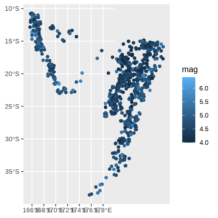
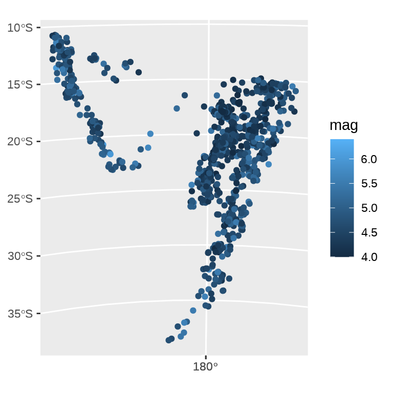
数据集 quakes_sf 已经准备了坐标参考系统,此时,coord_sf() 就会采用数据集相应的坐标参考系统,即 sf::st_crs(4326)。上图的左子图相当于:
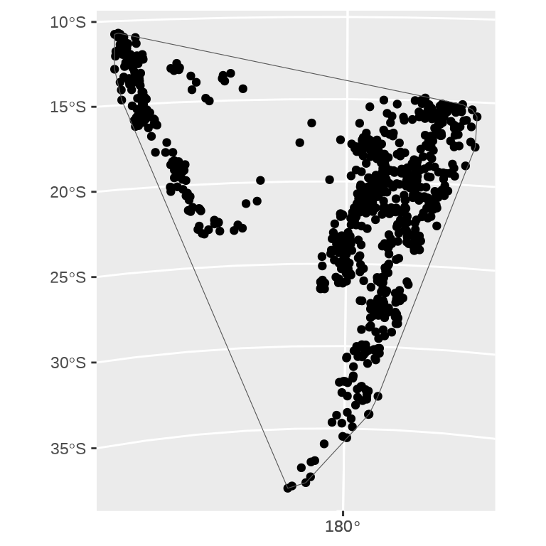
27.1.3 凸包操作
# 绘制点及其包络
plot(st_geometry(quakes_sf))
# 添加凸包曲线
plot(quakes_sfp_hull, add = TRUE)

ggplot() +
  geom_sf(data = quakes_sf) +
  geom_sf(data = quakes_sfp_hull, fill = NA) +
  coord_sf(crs = 3460, xlim = c(569061, 3008322), ylim = c(1603260, 4665206))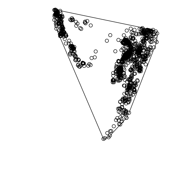
27.2 数据探索
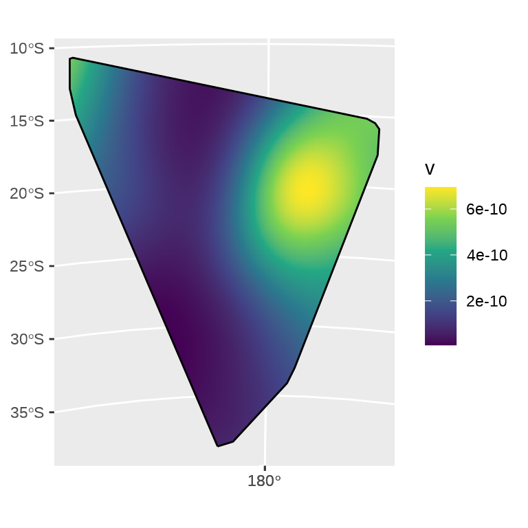
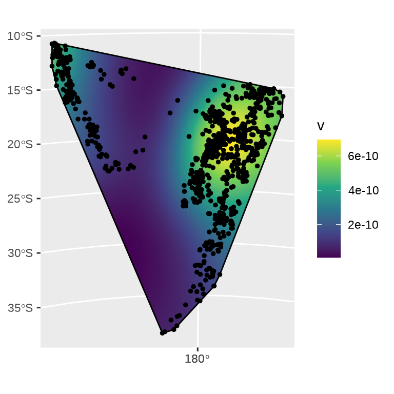
27.2.1 核密度估计
给定边界内的核密度估计与绘制热力图
#> Warning in as.ppp.sf(quakes_sf): only first attribute column is used for marks#> Warning: point-in-polygon test had difficulty with 1 point (total score not 0
#> or 1)27.2.2 绘制热力图
ggplot() +
  geom_sf(data = density_sf, aes(fill = v), col = NA) +
  scale_fill_viridis_c() +
  geom_sf(data = st_boundary(quakes_sfp_hull))

ggplot() +
  geom_sf(data = density_sf, aes(fill = v), col = NA) +
  scale_fill_viridis_c() +
  geom_sf(data = st_boundary(quakes_sfp_hull)) +
  geom_sf(data = quakes_sf, size = 1, col = "black")