library(StanHeaders)
library(ggplot2)
library(rstan)
# 将编译的 Stan 模型与代码文件放在一起
rstan_options(auto_write = TRUE)
# 如果CPU和内存足够,设置成与马尔科夫链一样多
options(mc.cores = max(c(floor(parallel::detectCores() / 2), 1L)))
# 调色板
custom_colors <- c(
  "#4285f4", # GoogleBlue
  "#34A853", # GoogleGreen
  "#FBBC05", # GoogleYellow
  "#EA4335"  # GoogleRed
)
rstan_ggtheme_options(
  panel.background = element_rect(fill = "white"),
  legend.position = "top"
)
rstan_gg_options(
  fill = "#4285f4", color = "white",
  pt_color = "#EA4335", chain_colors = custom_colors
)
library(bayesplot)35 分层正态模型
This is a bit like asking how should I tweak my sailboat so I can explore the ocean floor.
— Roger Koenker 1
乔治·博克斯说,所有的模型都是错的,但有些是有用的。在真实的数据面前,尽我们所能,结果发现没有最好的模型,只有更好的模型。总是需要自己去构造符合自己需求的模型及其实现,只有自己能够实现,才能在模型的海洋中畅快地遨游。
介绍分层正态模型的定义、结构、估计,分层正态模型与曲线生长模型的关系,分层正态模型与潜变量模型的关系,分层正态模型与线性混合效应的关系。以 rstan 包和 nlme 包拟合分层正态模型,说明 rstan 包的一些用法,比较贝叶斯和频率派方法拟合的结果,给出结果的解释。再对比 16 个不同的 R包实现,总结一般地使用经验,也体会不同 R 包的独特性。
35.1 rstan 包
本节以 8schools 数据为例介绍分层正态模型及 rstan 包实现,8schools 数据最早来自 Rubin (1981) ,分层正态模型如下:
\[ \begin{aligned} y_j &\sim \mathcal{N}(\theta_j,\sigma_j^2) \quad \theta_j = \mu + \tau \times \eta_j \\ \theta_j &\sim \mathcal{N}(\mu, \tau^2) \quad \eta_j \sim \mathcal{N}(0,1) \\ \mu &\sim \mathcal{N}(0, 100^2) \quad \tau \sim \mathrm{half\_normal}(0,100^2) \end{aligned} \]
其中,\(y_j,\sigma_j\) 是已知的观测数据,\(\theta_j\) 是模型参数, \(\eta_j\) 是服从标准正态分布的潜变量,\(\mu,\tau\) 是超参数,分别服从正态分布(将方差设置为很大的数,则变成弱信息先验或无信息均匀先验)和半正态分布(随机变量限制为正值)。
35.1.1 拟合模型
用 rstan 包来拟合模型,下面采用非中心的参数化表示,降低参数的相关性,减少发散的迭代次数,提高采样效率。
# 编译模型
eight_schools_fit <- stan(
  model_name = "eight_schools",
  # file = "code/eight_schools.stan",
  model_code = "
  // saved as eight_schools.stan
  data {
    int<lower=0> J;                // number of schools
    array[J] real y;               // estimated treatment effects
    array[J] real <lower=0> sigma; // standard error of effect estimates
  }
  parameters {
    real mu;                // population treatment effect
    real<lower=0> tau;      // standard deviation in treatment effects
    vector[J] eta;          // unscaled deviation from mu by school
  }
  transformed parameters {
    vector[J] theta = mu + tau * eta;        // school treatment effects
  }
  model {
    target += normal_lpdf(mu | 0, 100);
    target += normal_lpdf(tau | 0, 100);
    target += normal_lpdf(eta | 0, 1);  // prior log-density
    target += normal_lpdf(y | theta, sigma); // log-likelihood
  }
  ",
  data = list( # 观测数据
    J = 8,
    y = c(28, 8, -3, 7, -1, 1, 18, 12),
    sigma = c(15, 10, 16, 11, 9, 11, 10, 18)
  ),
  warmup = 1000, # 每条链预处理迭代次数
  iter = 2000,   # 每条链总迭代次数
  chains = 2,    # 马尔科夫链的数目
  cores = 2,     # 指定 CPU 核心数,可以给每条链分配一个
  verbose = FALSE, # 不显示迭代的中间过程
  refresh = 0,     # 不显示采样的进度
  seed = 20232023  # 设置随机数种子,不要使用 set.seed() 函数
)
#> Warning: There were 5 divergent transitions after warmup. See
#> https://mc-stan.org/misc/warnings.html#divergent-transitions-after-warmup
#> to find out why this is a problem and how to eliminate them.#> Warning: Examine the pairs() plot to diagnose sampling problems#> Warning: Tail Effective Samples Size (ESS) is too low, indicating posterior variances and tail quantiles may be unreliable.
#> Running the chains for more iterations may help. See
#> https://mc-stan.org/misc/warnings.html#tail-ess35.1.2 模型输出
用函数 print() 打印输出结果,保留 2 位小数。
#> Inference for Stan model: eight_schools.
#> 2 chains, each with iter=2000; warmup=1000; thin=1;
#> post-warmup draws per chain=1000, total post-warmup draws=2000.
#>
#>            mean se_mean   sd   2.5%    25%    50%    75%  97.5% n_eff Rhat
#> mu         7.42    0.48 5.81  -4.69   4.53   7.66  11.03  17.32   146 1.01
#> tau        6.79    0.58 6.66   0.17   2.34   5.24   8.96  25.21   132 1.02
#> eta[1]     0.37    0.02 0.93  -1.47  -0.25   0.41   1.02   2.06  1486 1.00
#> eta[2]     0.04    0.02 0.88  -1.69  -0.55   0.04   0.63   1.78  1853 1.01
#> eta[3]    -0.17    0.02 0.90  -1.92  -0.76  -0.19   0.45   1.62  1940 1.00
#> eta[4]    -0.01    0.02 0.87  -1.74  -0.59  -0.02   0.60   1.66  1356 1.00
#> eta[5]    -0.32    0.02 0.88  -2.08  -0.89  -0.34   0.25   1.50  1395 1.00
#> eta[6]    -0.17    0.02 0.86  -1.93  -0.76  -0.16   0.38   1.60  1709 1.00
#> eta[7]     0.35    0.02 0.89  -1.56  -0.24   0.40   0.93   2.04  1492 1.00
#> eta[8]     0.09    0.02 0.93  -1.73  -0.50   0.09   0.70   1.98  1759 1.00
#> theta[1]  11.02    0.21 8.09  -3.03   5.81  10.15  14.95  31.74  1421 1.00
#> theta[2]   7.86    0.14 6.46  -4.79   3.84   7.74  11.85  20.63  2055 1.00
#> theta[3]   5.86    0.45 8.41 -12.96   1.93   6.68  10.80  19.85   343 1.01
#> theta[4]   7.61    0.14 6.39  -4.98   3.58   7.78  11.50  20.37  2024 1.00
#> theta[5]   5.00    0.20 6.51  -9.71   1.29   5.59   9.34  16.59  1090 1.00
#> theta[6]   6.06    0.27 6.80  -9.09   2.34   6.52  10.53  17.94   638 1.00
#> theta[7]  10.53    0.18 6.63  -1.23   5.88  10.03  14.56  25.23  1367 1.00
#> theta[8]   8.27    0.23 7.72  -7.24   3.55   8.32  12.76  23.96  1104 1.00
#> lp__     -50.59    0.11 2.62 -56.71 -52.14 -50.38 -48.76 -46.20   586 1.00
#>
#> Samples were drawn using NUTS(diag_e) at Sun Dec 10 15:14:03 2023.
#> For each parameter, n_eff is a crude measure of effective sample size,
#> and Rhat is the potential scale reduction factor on split chains (at
#> convergence, Rhat=1).
值得一提,数据有限而且规律不明确,数据隐含的信息不是很多,则先验分布的情况将会对参数估计结果产生很大影响。Stan 默认采用无信息的先验分布,当使用非常弱的信息先验时,结果就非常不同了。提取任意一个参数的结果,如查看参数 \(\tau\) 的 95% 置信区间。
#> Inference for Stan model: eight_schools.
#> 2 chains, each with iter=2000; warmup=1000; thin=1;
#> post-warmup draws per chain=1000, total post-warmup draws=2000.
#>
#>     mean se_mean   sd 2.5% 97.5% n_eff Rhat
#> tau 6.79    0.58 6.66 0.17 25.21   132 1.02
#>
#> Samples were drawn using NUTS(diag_e) at Sun Dec 10 15:14:03 2023.
#> For each parameter, n_eff is a crude measure of effective sample size,
#> and Rhat is the potential scale reduction factor on split chains (at
#> convergence, Rhat=1).
从迭代抽样数据获得与 print(fit) 一样的结果。以便后续对原始采样数据做任意的进一步分析。rstan 包扩展泛型函数 summary() 以支持对 stanfit 数据对象汇总,输出各个参数分链条和合并链条的后验分布结果。
35.1.3 操作数据
抽取数据对象 eight_schools_fit 中的采样数据,合并几条马氏链的结果,返回的结果是一个列表。
返回列表中的每个元素是一个数组,标量参数对应一维数组,向量参数对应二维数组。
#> List of 5
#>  $ mu   : num [1:2000(1d)] 5.75 7.63 19.11 16.11 10.39 ...
#>   ..- attr(*, "dimnames")=List of 1
#>   .. ..$ iterations: NULL
#>  $ tau  : num [1:2000(1d)] 10.16 8.47 17.3 4.1 6.47 ...
#>   ..- attr(*, "dimnames")=List of 1
#>   .. ..$ iterations: NULL
#>  $ eta  : num [1:2000, 1:8] 1.556 1.356 0.369 -0.433 1.293 ...
#>   ..- attr(*, "dimnames")=List of 2
#>   .. ..$ iterations: NULL
#>   .. ..$           : NULL
#>  $ theta: num [1:2000, 1:8] 21.6 19.1 25.5 14.3 18.8 ...
#>   ..- attr(*, "dimnames")=List of 2
#>   .. ..$ iterations: NULL
#>   .. ..$           : NULL
#>  $ lp__ : num [1:2000(1d)] -47.8 -47.4 -48.5 -52.1 -48.1 ...
#>   ..- attr(*, "dimnames")=List of 1
#>   .. ..$ iterations: NULL
对于列表,适合用函数 lapply() 配合算术函数计算 \(\mu,\tau\) 等参数的均值。
fun_mean <- function(x) {
  if (length(dim(x)) > 1) {
    apply(x, 2, mean)
  } else {
    mean(x)
  }
}
lapply(eight_schools_sim, FUN = fun_mean)
#> $mu
#> [1] 7.42289
#>
#> $tau
#> [1] 6.785338
#>
#> $eta
#> [1] 0.36786577 0.03963007 -0.16870656 -0.01330852 -0.32387749 -0.17455433
#> [7] 0.34977497 0.09338187
#>
#> $theta
#> [1] 11.021965 7.864931 5.859438 7.610153 5.004556 6.062694 10.531080
#> [8] 8.272096
#>
#> $lp__
#> [1] -50.59453类似地,计算 \(\mu,\tau\) 等参数的分位点。
fun_quantile <- function(x, probs) {
  if (length(dim(x)) > 1) {
    t(apply(x, 2, quantile, probs = probs))
  } else {
    quantile(x, probs = probs)
  }
}
lapply(eight_schools_sim, fun_quantile, probs = c(2.5, 25, 50, 75, 97.5) / 100)
#> $mu
#> 2.5% 25% 50% 75% 97.5%
#> -4.688686 4.525320 7.660881 11.026361 17.316378
#>
#> $tau
#> 2.5% 25% 50% 75% 97.5%
#> 0.1725007 2.3406296 5.2397766 8.9599336 25.2140896
#>
#> $eta
#>
#> 2.5% 25% 50% 75% 97.5%
#> [1,] -1.472725 -0.2463519 0.40944442 1.0169994 2.058549
#> [2,] -1.692349 -0.5484956 0.03527577 0.6313437 1.779431
#> [3,] -1.915337 -0.7614554 -0.18762414 0.4470704 1.622897
#> [4,] -1.740432 -0.5895913 -0.01766319 0.5977618 1.658543
#> [5,] -2.077877 -0.8882916 -0.33870235 0.2505137 1.496111
#> [6,] -1.927826 -0.7605602 -0.16412062 0.3800892 1.598579
#> [7,] -1.560540 -0.2353192 0.39542982 0.9304768 2.036753
#> [8,] -1.730880 -0.5037635 0.09230484 0.6956278 1.975779
#>
#> $theta
#>
#> 2.5% 25% 50% 75% 97.5%
#> [1,] -3.030548 5.811833 10.152085 14.950004 31.74400
#> [2,] -4.786133 3.836380 7.742984 11.846956 20.63119
#> [3,] -12.957206 1.925727 6.679549 10.798270 19.84788
#> [4,] -4.978866 3.581948 7.779776 11.496501 20.37373
#> [5,] -9.713078 1.293159 5.589891 9.344892 16.58744
#> [6,] -9.086488 2.339967 6.515114 10.527118 17.94399
#> [7,] -1.232794 5.879803 10.032427 14.559353 25.23035
#> [8,] -7.244677 3.545208 8.324813 12.764714 23.95992
#>
#> $lp__
#> 2.5% 25% 50% 75% 97.5%
#> -56.71080 -52.13763 -50.38239 -48.76393 -46.2035035.1.4 采样诊断
获取马尔科夫链迭代点列数据
eight_schools_sim 是一个三维数组,1000(次迭代)* 2 (条链)* 19(个参数)。如果 permuted = TRUE 则会合并马氏链的迭代结果,变成一个列表。
#> [1] "array"#> num [1:1000, 1:2, 1:19] 8.65 12.09 6.11 6.11 17.6 ...
#> - attr(*, "dimnames")=List of 3
#> ..$ iterations: NULL
#> ..$ chains : chr [1:2] "chain:1" "chain:2"
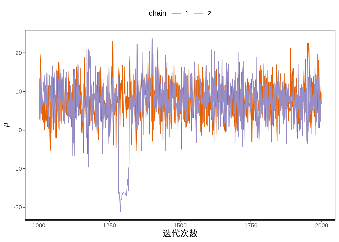
#> ..$ parameters: chr [1:19] "mu" "tau" "eta[1]" "eta[2]" ...提取参数 \(\mu\) 的迭代点列,绘制迭代轨迹。
eight_schools_mu_sim <- eight_schools_sim[, , "mu"]
matplot(
  eight_schools_mu_sim, xlab = "迭代次数", ylab = expression(mu),
  type = "l", lty = "solid", col = custom_colors
)
abline(h = apply(eight_schools_mu_sim, 2, mean), col = custom_colors)
legend(
  "topleft", legend = paste("chain", 1:2), box.col = "white",
  inset = 0.01, lty = "solid", horiz = TRUE, col = custom_colors
)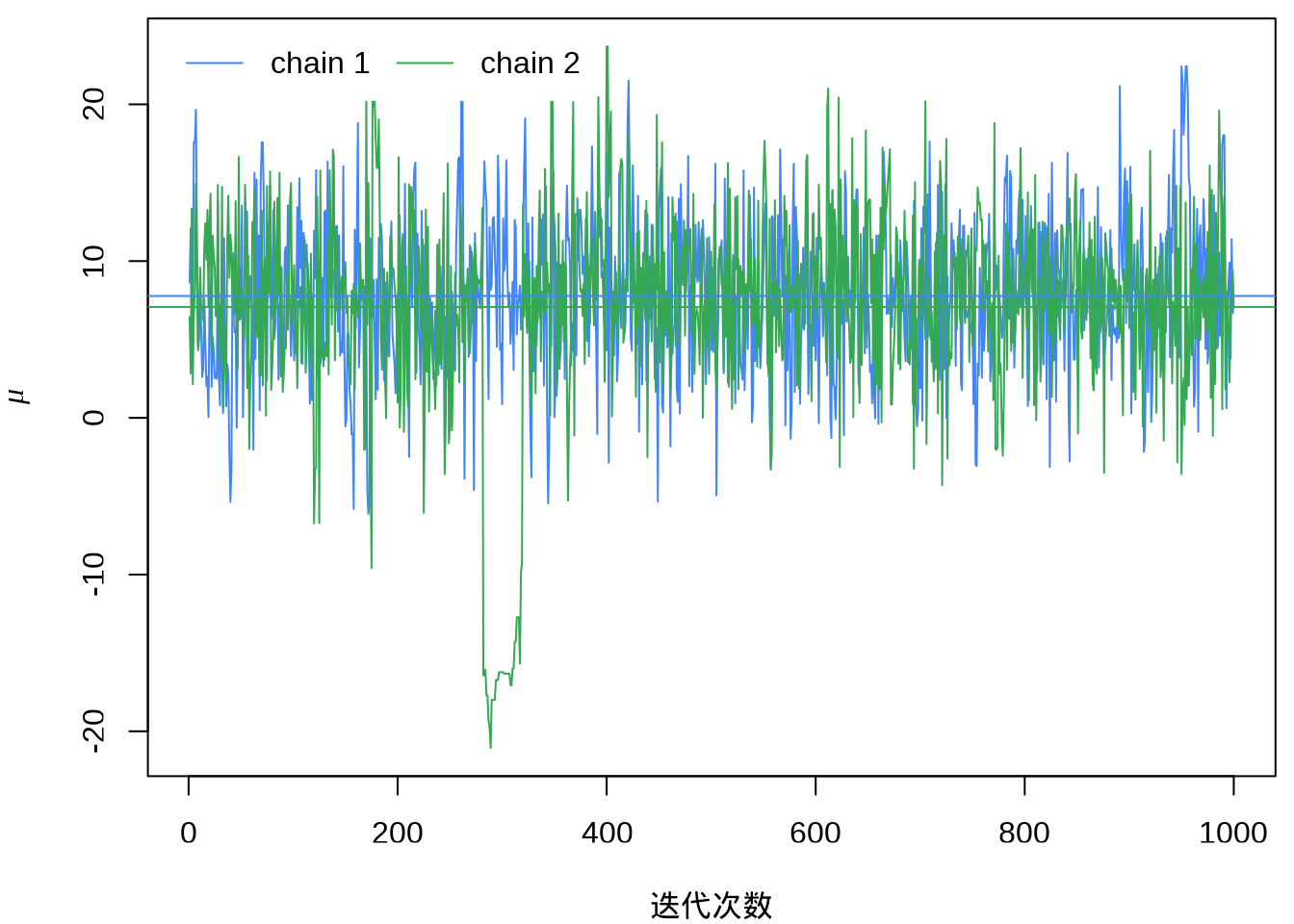
也可以使用 rstan 包提供的函数 traceplot() 或者 stan_trace() 绘制参数的迭代轨迹图。
35.1.5 后验分布
可以用函数 stan_hist() 或 stan_dens() 绘制后验分布图。下图分别展示参数 \(\mu\)、\(\tau\) 的直方图,以及二者的散点图,参数 \(\mu\) 的后验概率密度分布图。
p1 <- stan_hist(eight_schools_fit, pars = c("mu","tau"), bins = 30)
p2 <- stan_scat(eight_schools_fit, pars = c("mu","tau"), size = 1) +
  labs(x = expression(mu), y = expression(tau))
p3 <- stan_dens(eight_schools_fit, pars = "mu") + labs(x = expression(mu))
library(patchwork)
p1 / (p2 + p3)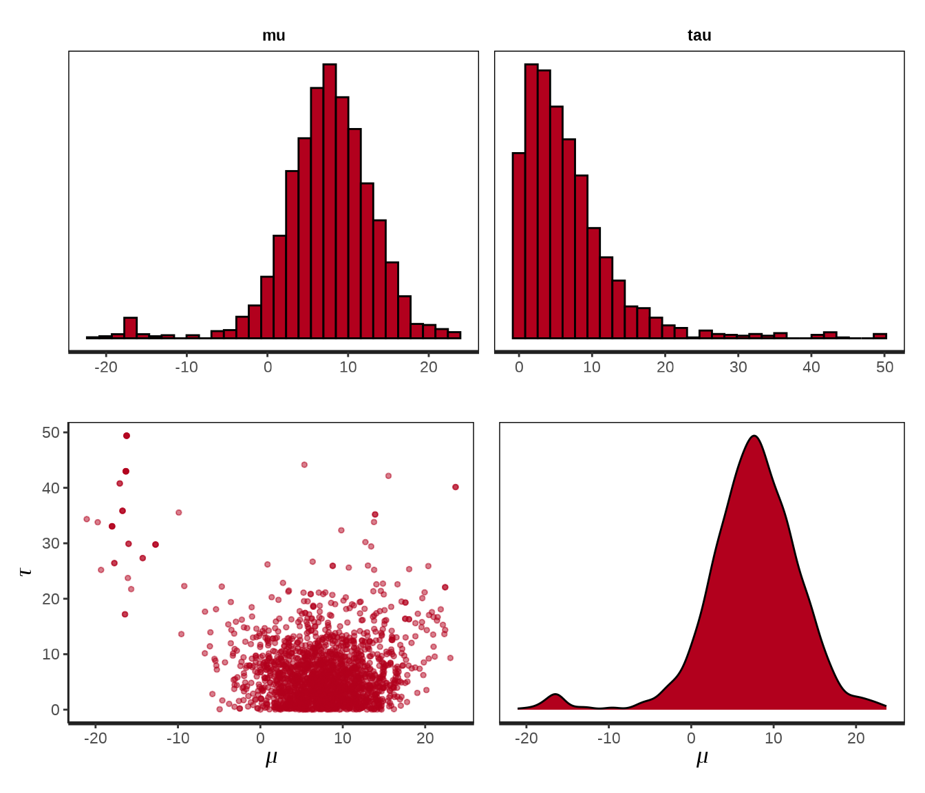
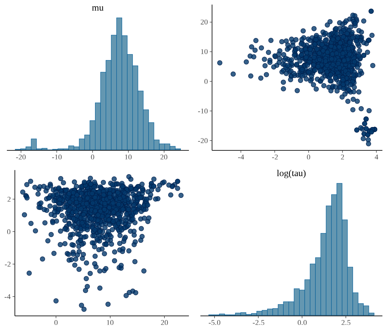
相比于 rstan 包,bayesplot 包可视化能力更强,支持对特定的参数做变换。bayesplot 包的函数 mcmc_pairs() 以矩阵图展示多个参数的分布,下图展示参数 \(\mu\),\(\log(\tau)\) 后验分布图。但是,这些函数都固定了一些标题,不能修改。
35.2 其它 R 包
35.2.1 nlme
接下来,用 nlme 包拟合模型。
首先,调用 nlme 包的函数 lme() 拟合模型。
library(nlme)
fit_lme <- lme(y ~ 1, random = ~ 1 | g, weights = varFixed(~ sigma^2), method = "REML")
summary(fit_lme)
#> Linear mixed-effects model fit by REML
#> Data: NULL
#> AIC BIC logLik
#> 60.21091 60.04864 -27.10546
#>
#> Random effects:
#> Formula: ~1 | g
#> (Intercept) Residual
#> StdDev: 2.917988 0.780826
#>
#> Variance function:
#> Structure: fixed weights
#> Formula: ~sigma^2
#> Fixed effects: y ~ 1
#> Value Std.Error DF t-value p-value
#> (Intercept) 7.785729 3.368082 8 2.311621 0.0496
#>
#> Standardized Within-Group Residuals:
#> Min Q1 Med Q3 Max
#> -1.06635035 -0.73588511 -0.02896764 0.50254917 1.62502386
#>
#> Number of Observations: 8
#> Number of Groups: 8随机效应的标准差 2.917988 ,随机效应部分的估计
#>   (Intercept)
#> 1  1.18135690
#> 2  0.02625714
#> 3 -0.55795543
#> 4 -0.08130333
#> 5 -1.29202240
#> 6 -0.70215328
#> 7  1.25167648
#> 8  0.17414393
类比 Stan 输出结果中的 \(\theta\) 向量,每个学校的成绩估计
35.2.2 lme4
接着,采用 lme4 包拟合模型,发现 lme4 包获得与 nlme 包一样的结果。
control <- lme4::lmerControl(
  check.conv.singular = "ignore",
  check.nobs.vs.nRE = "ignore",
  check.nobs.vs.nlev = "ignore"
)
fit_lme4 <- lme4::lmer(y ~ 1 + (1 | g), weights = 1 / sigma^2, control = control, REML = TRUE)
summary(fit_lme4)
#> Linear mixed model fit by REML ['lmerMod']
#> Formula: y ~ 1 + (1 | g)
#> Weights: 1/sigma^2
#> Control: control
#>
#> REML criterion at convergence: 54.2
#>
#> Scaled residuals:
#> Min 1Q Median 3Q Max
#> -1.06635 -0.73589 -0.02897 0.50255 1.62502
#>
#> Random effects:
#> Groups Name Variance Std.Dev.
#> g (Intercept) 8.5145 2.9180
#> Residual 0.6097 0.7808
#> Number of obs: 8, groups: g, 8
#>
#> Fixed effects:
#> Estimate Std. Error t value
#> (Intercept) 7.786 3.368 2.31235.2.3 blme
下面使用 blme 包 (Chung 等 2013) ,blme 包基于 lme4 包,参数估计结果完全一致。
# the mode should be at the boundary of the space.

fit_blme <- blme::blmer(
  y ~ 1 + (1 | g), control = control, REML = TRUE,
  cov.prior = NULL, weights = 1 / sigma^2
)
summary(fit_blme)
#> Prior dev : 0
#>
#> Linear mixed model fit by REML ['blmerMod']
#> Formula: y ~ 1 + (1 | g)
#> Weights: 1/sigma^2
#> Control: control
#>
#> REML criterion at convergence: 54.2
#>
#> Scaled residuals:
#> Min 1Q Median 3Q Max
#> -1.06635 -0.73589 -0.02897 0.50255 1.62502
#>
#> Random effects:
#> Groups Name Variance Std.Dev.
#> g (Intercept) 8.5145 2.9180
#> Residual 0.6097 0.7808
#> Number of obs: 8, groups: g, 8
#>
#> Fixed effects:
#> Estimate Std. Error t value
#> (Intercept) 7.786 3.368 2.31235.2.4 MCMCglmm
MCMCglmm 包 (Hadfield 2010) 采用 MCMC 算法拟合数据。
schools <- data.frame(y = y, sigma = sigma, g = g)
schools$g <- as.factor(schools$g)
# inverse-gamma prior with scale and shape equal to 0.001
prior1 <- list(
  R = list(V = diag(schools$sigma^2), fix = 1),
  G = list(G1 = list(V = 1, nu = 0.002))
)
# 为可重复
set.seed(20232023)
# 拟合模型
fit_mcmc <- MCMCglmm::MCMCglmm(
  y ~ 1, random = ~g, rcov = ~ idh(g):units,
  data = schools, prior = prior1, verbose = FALSE
)
# 输出结果
summary(fit_mcmc)
#>
#> Iterations = 3001:12991
#> Thinning interval = 10
#> Sample size = 1000
#>
#> DIC: -98.07615
#>
#> G-structure: ~g
#>
#> post.mean l-95% CI u-95% CI eff.samp
#> g 11.23 0.0004247 68.57 361.3
#>
#> R-structure: ~idh(g):units
#>
#> post.mean l-95% CI u-95% CI eff.samp
#> g1.units 225 225 225 0
#> g2.units 100 100 100 0
#> g3.units 256 256 256 0
#> g4.units 121 121 121 0
#> g5.units 81 81 81 0
#> g6.units 121 121 121 0
#> g7.units 100 100 100 0
#> g8.units 324 324 324 0
#>
#> Location effects: y ~ 1
#>
#> post.mean l-95% CI u-95% CI eff.samp pMCMC
#> (Intercept) 7.6938 -0.5149 15.3275 1023 0.062 .
#> ---
#> Signif. codes: 0 '***' 0.001 '**' 0.01 '*' 0.05 '.' 0.1 ' ' 1R-structure 表示残差方差,这是已知的参数。G-structure 表示随机截距的方差,Location effects 表示固定效应的截距。截距和 nlme 包的结果很接近。
35.2.5 cmdstanr
一般地,rstan 包使用的 stan 框架版本低于 cmdstanr 包,从 rstan 包切换到 cmdstanr 包,需要注意语法、函数的变化。rstan 和 cmdstanr 使用的 Stan 版本不同导致参数估计结果不同,结果可重复的条件非常苛刻,详见 Stan 参考手册。在都是较新的版本时,Stan 代码不需要做改动,如下:
data {
  int<lower=0> J; // 学校数目
  array[J] real y; // 测试效果的预测值
  array[J] real <lower=0> sigma; // 测试效果的标准差
}
parameters {
  real mu;
  real<lower=0> tau;
  vector[J] eta;
}
transformed parameters {
  vector[J] theta;
  theta = mu + tau * eta;
}
model {
  target += normal_lpdf(mu | 0, 100);
  target += normal_lpdf(tau | 0, 100);
  target += normal_lpdf(eta | 0, 1);
  target += normal_lpdf(y | theta, sigma);
}
此处,给参数 \(\mu,\tau\) 添加了非常弱(模糊)的先验,结果将出现较大不同。
eight_schools_dat <- list(
  J = 8,
  y = c(28, 8, -3, 7, -1, 1, 18, 12),
  sigma = c(15, 10, 16, 11, 9, 11, 10, 18)
)
library(cmdstanr)
mod_eight_schools <- cmdstan_model(
  stan_file = "code/eight_schools.stan",
  compile = TRUE, cpp_options = list(stan_threads = TRUE)
)
fit_eight_schools <- mod_eight_schools$sample(
  data = eight_schools_dat, # 数据
  chains = 2,            # 总链条数
  parallel_chains = 2,   # 并行数目
  iter_warmup = 1000,    # 每条链预处理的迭代次数
  iter_sampling = 1000,  # 每条链采样的迭代次数
  threads_per_chain = 2, # 每条链设置 2 个线程
  seed = 20232023,       # 随机数种子
  show_messages = FALSE, # 不显示消息
  refresh = 0 # 不显示采样迭代的进度
)
结果保留 3 位有效数字,模型输出如下:
#> # A tibble: 19 × 10
#>    variable     mean   median    sd   mad      q5    q95  rhat ess_bulk ess_tail
#>    <chr>       <dbl>    <dbl> <dbl> <dbl>   <dbl>  <dbl> <dbl>    <dbl>    <dbl>
#>  1 lp__     -50.7    -50.4    2.54  2.43  -55.3   -46.9  1.00      515.     891.
#>  2 mu         7.92     7.85   4.71  4.55    0.133  15.7  1.00     1209.     723.
#>  3 tau        6.21     5.04   5.04  4.53    0.519  15.9  1.00      683.     843.
#>  4 eta[1]     0.324    0.334  0.982 0.976  -1.34    1.91 1.00     1855.    1148.
#>  5 eta[2]    -0.0394  -0.0396 0.852 0.860  -1.49    1.36 1.00     1882.    1405.
#>  6 eta[3]    -0.190   -0.193  0.947 0.911  -1.72    1.38 1.00     1734.    1242.
#>  7 eta[4]    -0.0307  -0.0261 0.879 0.865  -1.49    1.40 1.00     1590.    1209.
#>  8 eta[5]    -0.341   -0.369  0.896 0.841  -1.78    1.20 1.00     1687.    1370.
#>  9 eta[6]    -0.239   -0.233  0.904 0.897  -1.71    1.28 1.00     1588.    1111.
#> 10 eta[7]     0.321    0.345  0.909 0.895  -1.20    1.71 0.999    1738.    1196.
#> 11 eta[8]     0.0656   0.0700 0.952 0.965  -1.46    1.67 1.00     1847.    1296.
#> 12 theta[1]  10.7      9.48   8.26  6.58   -0.523  26.3  1.00     1866.    1225.
#> 13 theta[2]   7.61     7.54   6.14  5.70   -2.13   17.8  1.00     2351.    1734.
#> 14 theta[3]   6.15     6.50   7.38  5.99   -7.06   17.7  1.00     1874.    1252.
#> 15 theta[4]   7.55     7.65   6.19  5.79   -2.65   17.6  1.00     2050.    1436.
#> 16 theta[5]   5.17     5.65   6.29  5.86   -6.25   14.6  1.00     2072.    1656.
#> 17 theta[6]   6.01     6.50   6.87  5.98   -6.68   16.6  1.00     1802.    1251.
#> 18 theta[7]  10.4      9.89   6.52  5.95    0.518  22.1  1.00     1607.    1513.
#> 19 theta[8]   8.38     8.08   7.68  6.27   -3.65   21.0  1.00     1772.    1500.
模型采样过程的诊断结果如下:
#> Warning: 2 of 2000 (0.0%) transitions ended with a divergence.
#> See https://mc-stan.org/misc/warnings for details.
#> $num_divergent
#> [1] 0 2
#>
#> $num_max_treedepth
#> [1] 0 0
#>
#> $ebfmi
#> [1] 1.0218599 0.8735072分层模型的参数 \(\mu,\log(\tau)\) 的后验联合分布呈现经典的漏斗状。
bayesplot::mcmc_scatter(
  fit_eight_schools$draws(), pars = c("mu", "tau"),
  transform = list(tau = "log"), size = 2
) + labs(x = "$\\mu$", y = "$\\log(\\tau)$")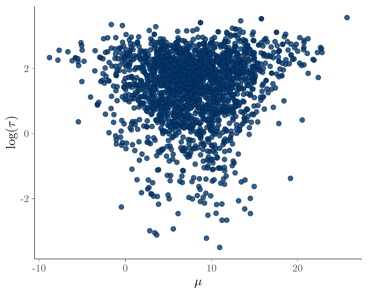
对于调用 cmdstanr 包拟合的模型,适合用 bayesplot 包来可视化后验分布和诊断采样。
35.3 案例:rats 数据
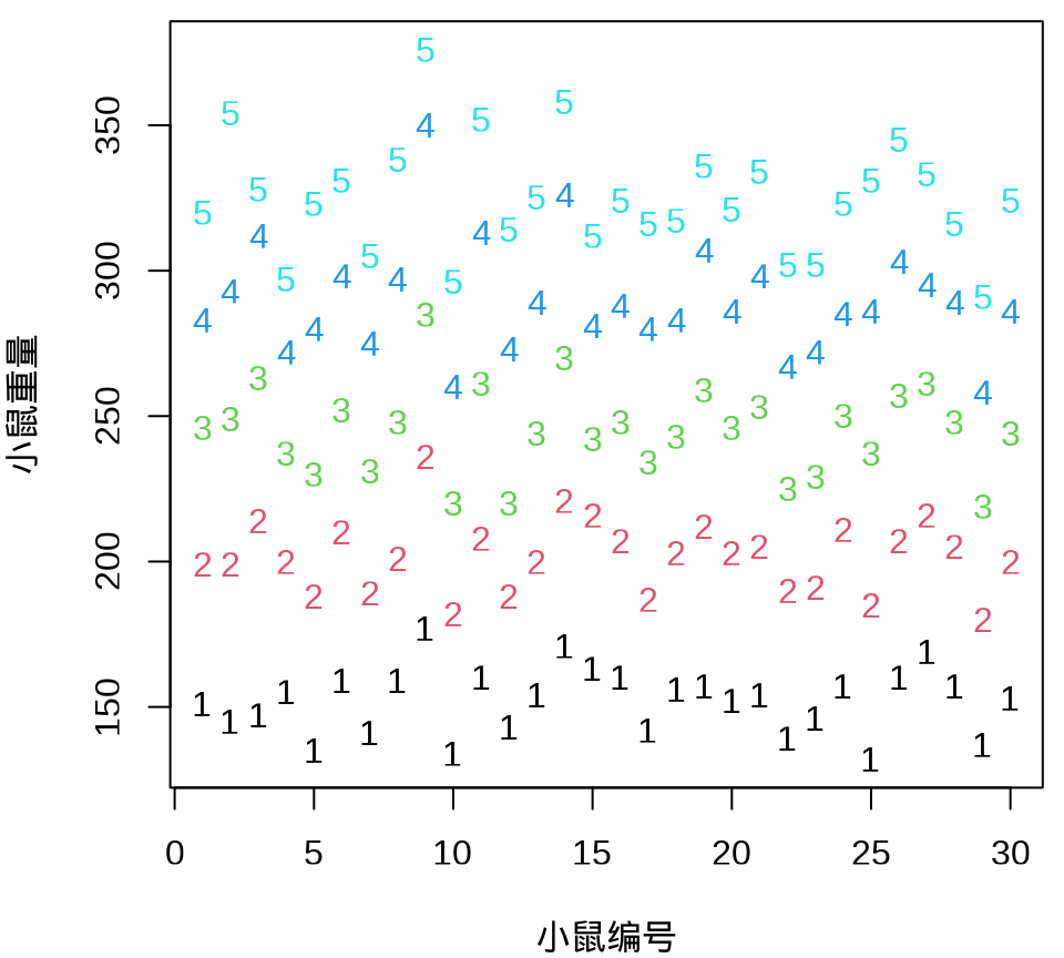
rats 数据最早来自 Gelfand 等 (1990) ,记录 30 只小鼠每隔一周的重量,一共进行了 5 周。第一次记录是小鼠第 8 天的时候,第二次测量记录是第 15 天的时候,一直持续到第 36 天。下面在 R 环境中准备数据。
# 总共 30 只老鼠
N <- 30
# 总共进行 5 周
T <- 5
# 小鼠重量
y <- structure(c(
  151, 145, 147, 155, 135, 159, 141, 159, 177, 134,
  160, 143, 154, 171, 163, 160, 142, 156, 157, 152, 154, 139, 146,
  157, 132, 160, 169, 157, 137, 153, 199, 199, 214, 200, 188, 210,
  189, 201, 236, 182, 208, 188, 200, 221, 216, 207, 187, 203, 212,
  203, 205, 190, 191, 211, 185, 207, 216, 205, 180, 200, 246, 249,
  263, 237, 230, 252, 231, 248, 285, 220, 261, 220, 244, 270, 242,
  248, 234, 243, 259, 246, 253, 225, 229, 250, 237, 257, 261, 248,
  219, 244, 283, 293, 312, 272, 280, 298, 275, 297, 350, 260, 313,
  273, 289, 326, 281, 288, 280, 283, 307, 286, 298, 267, 272, 285,
  286, 303, 295, 289, 258, 286, 320, 354, 328, 297, 323, 331, 305,
  338, 376, 296, 352, 314, 325, 358, 312, 324, 316, 317, 336, 321,
  334, 302, 302, 323, 331, 345, 333, 316, 291, 324
), .Dim = c(30, 5))
# 第几天
x <- c(8.0, 15.0, 22.0, 29.0, 36.0)
xbar <- 22.0
重复测量的小鼠重量数据 rats 如下 表格 35.1 所示。
| 第 8 天 | 第 15 天 | 第 22 天 | 第 29 天 | 第 36 天 | |
|---|---|---|---|---|---|
| 1 | 151 | 199 | 246 | 283 | 320 |
| 2 | 145 | 199 | 249 | 293 | 354 |
| 3 | 147 | 214 | 263 | 312 | 328 |
| 4 | 155 | 200 | 237 | 272 | 297 |
| 5 | 135 | 188 | 230 | 280 | 323 |
| 6 | 159 | 210 | 252 | 298 | 331 |
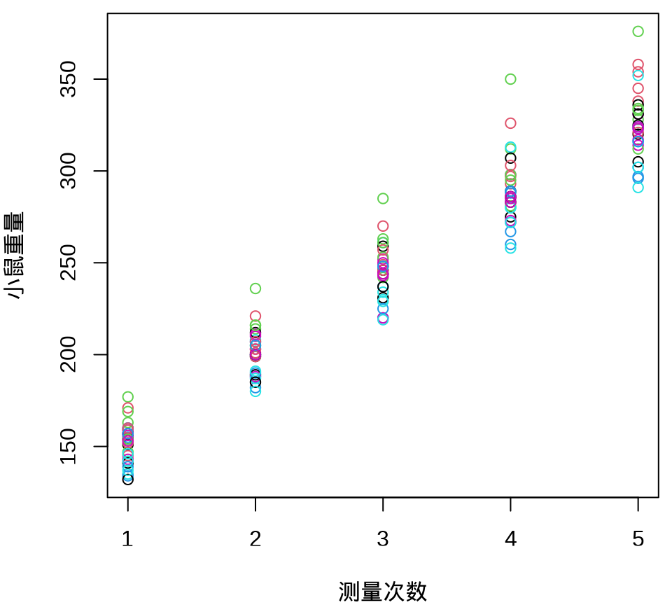
小鼠重量数据的分布和变化情况见下图,由图可以假定 30 只小鼠的重量服从正态分布,而30 只小鼠的重量呈现一种线性增长趋势。
35.4 频率派方法
35.4.1 nlme
nlme 包适合长格式的数据,因此,先将小鼠数据整理成长格式。
将 30 只小鼠的重量变化及回归曲线画出来,发现各只小鼠的回归线的斜率几乎一样,截距略有不同。不同小鼠的出生重量是不同,前面 Stan 采用变截距变斜率的混合效应模型拟合数据。
ggplot(data = rats_data, aes(x = days, y = weight)) +
  geom_point() +
  geom_smooth(formula = "y ~ x", method = "lm", se = FALSE) +
  theme_bw() +
  facet_wrap(facets = ~rats, labeller = "label_both", ncol = 6) +
  labs(x = "第几天", y = "重量")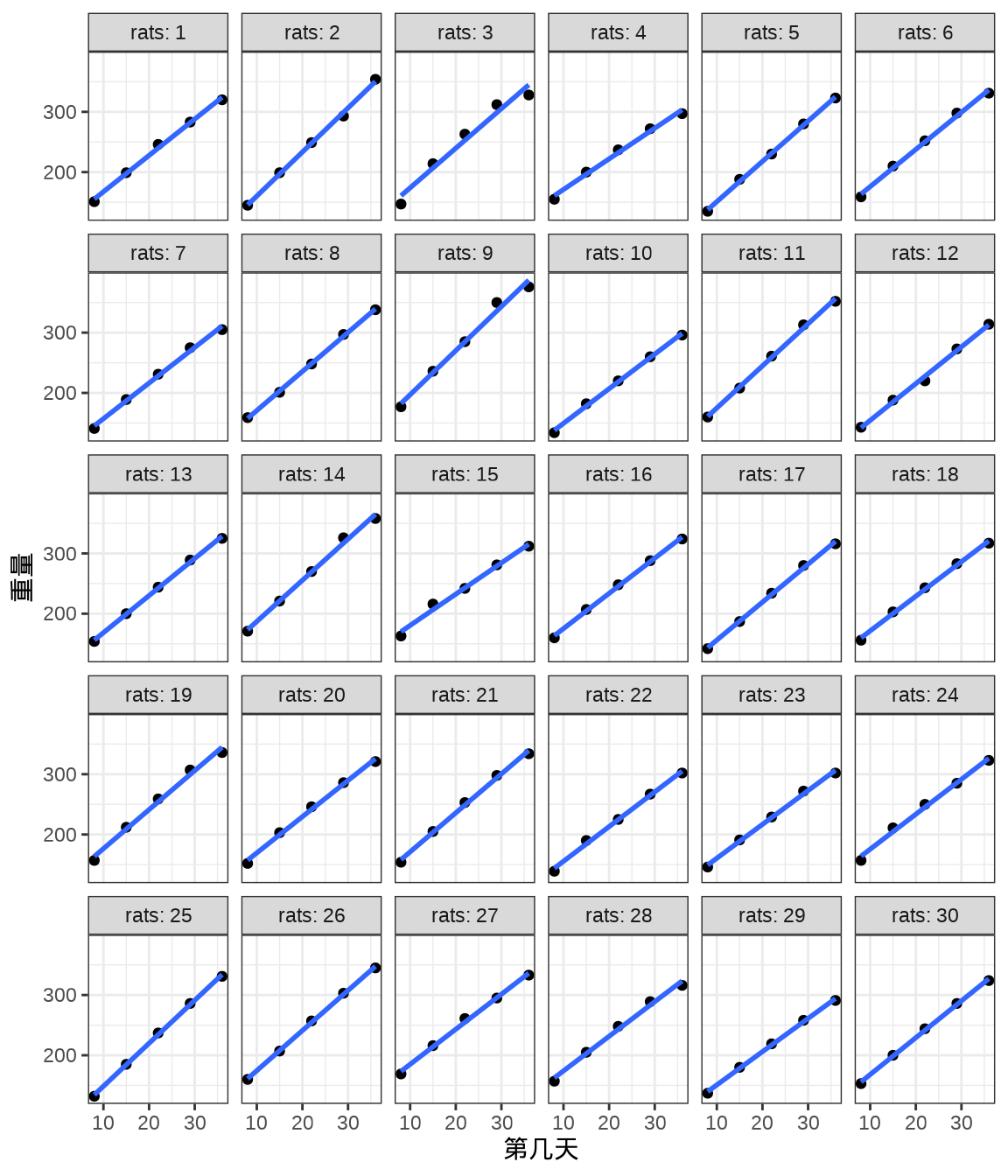
小鼠的重量随时间增长,不同小鼠的情况又会有所不同。作为一个参照,首先考虑变截距的随机效应模型。
\[ y_{ij} = \beta_0 + \beta_1 * x_j + \alpha_i + \epsilon_{ij}, \quad i = 1,2,\ldots,30. \quad j = 1,2,3,4,5 \]
其中,\(y_{ij}\) 表示第 \(i\) 只小鼠在第 \(j\) 次测量的重量,一共 30 只小鼠,共测量了 5 次。固定效应部分是 \(\beta_0\) 和 \(\beta_1\) ,分别表示截距和斜率。随机效应部分是 \(\alpha_i\) 和 \(\epsilon_{ij}\) ,分别服从正态分布\(\alpha_i \sim \mathcal{N}(0, \sigma^2_{\alpha})\) 和 \(\epsilon_{ij} \sim \mathcal{N}(0, \sigma^2_{\epsilon})\) 。\(\sigma^2_{\alpha}\) 和 \(\sigma^2_{\epsilon}\) 分别表示组间方差(group level)和组内方差(individual level)。
library(nlme)
rats_lme0 <- lme(data = rats_data, fixed = weight ~ days, random = ~ 1 | rats)
summary(rats_lme0)
#> Linear mixed-effects model fit by REML
#> Data: rats_data
#> AIC BIC logLik
#> 1145.302 1157.29 -568.6508
#>
#> Random effects:
#> Formula: ~1 | rats
#> (Intercept) Residual
#> StdDev: 14.03351 8.203811
#>
#> Fixed effects: weight ~ days
#> Value Std.Error DF t-value p-value
#> (Intercept) 106.56762 3.0379720 119 35.07854 0
#> days 6.18571 0.0676639 119 91.41824 0
#> Correlation:
#> (Intr)
#> days -0.49
#>
#> Standardized Within-Group Residuals:
#> Min Q1 Med Q3 Max
#> -2.7388198 -0.4770046 0.1261342 0.5634904 2.9981636
#>
#> Number of Observations: 150
#> Number of Groups: 30当然,若考虑不同小鼠的生长速度不同(变化不是很大),可用变截距和变斜率的随机效应模型表示生长曲线模型,下面加载 nlme 包调用函数 lme() 拟合该模型。
library(nlme)
rats_lme <- lme(data = rats_data, fixed = weight ~ days, random = ~ days | rats)
summary(rats_lme)
#> Linear mixed-effects model fit by REML
#> Data: rats_data
#> AIC BIC logLik
#> 1107.373 1125.357 -547.6867
#>
#> Random effects:
#> Formula: ~days | rats
#> Structure: General positive-definite, Log-Cholesky parametrization
#> StdDev Corr
#> (Intercept) 10.7426861 (Intr)
#> days 0.5105416 -0.159
#> Residual 6.0146565
#>
#> Fixed effects: weight ~ days
#> Value Std.Error DF t-value p-value
#> (Intercept) 106.56762 2.2976339 119 46.38146 0
#> days 6.18571 0.1055906 119 58.58204 0
#> Correlation:
#> (Intr)
#> days -0.343
#>
#> Standardized Within-Group Residuals:
#> Min Q1 Med Q3 Max
#> -2.6370819 -0.5394887 0.1187661 0.4927193 2.6090706
#>
#> Number of Observations: 150
#> Number of Groups: 30模型输出结果中,固定效应中的截距项 (Intercept) 对应 106.56762,斜率 days 对应 6.18571。Stan 模型中截距参数 alpha0 的后验估计是 106.332,斜率参数 beta_c 的后验估计是 6.188。对比 Stan 和 nlme 包的拟合结果,可以发现贝叶斯和频率方法的结果是非常接近的。截距参数 alpha0 可以看作小鼠的初始(出生)重量,斜率参数 beta_c 可以看作小鼠的生长率 growth rate。
函数 lme() 的输出结果中,随机效应的随机截距标准差 10.7425835,对应 tau_alpha,表示每个小鼠的截距偏移量的波动。而随机斜率的标准差为 0.5105447,对应 tau_beta,相对随机截距标准差来说很小。残差标准差为 6.0146608,对应 tau_c,表示与小鼠无关的剩余量的波动,比如测量误差。总之,和 Stan 的结果有所不同,但相去不远。主要是前面的 Stan 模型没有考虑随机截距和随机斜率之间的相关性,这可以进一步调整 (Sorensen, Hohenstein, 和 Vasishth 2016) 。
#> Approximate 95% confidence intervals
#>
#>  Fixed effects:
#>                  lower       est.      upper
#> (Intercept) 102.018074 106.567619 111.117164
#> days          5.976634   6.185714   6.394794
#>
#>  Random Effects:
#>   Level: rats
#>                            lower       est.      upper
#> sd((Intercept))        7.5158665 10.7426861 15.3548900
#> sd(days)               0.3659669  0.5105416  0.7122303
#> cor((Intercept),days) -0.5664773 -0.1590228  0.3109097
#>
#>  Within-group standard error:
#>    lower     est.    upper
#> 5.197149 6.014656 6.960757
Stan 输出中,截距项 alpha、斜率项 beta 参数的标准差分别是 tau_alpha 和 tau_beta ,残差标准差参数 tau_c 的估计为 6.1。简单起见,没有考虑截距项和斜率项的相关性,即不考虑小鼠出生时的重量和生长率的相关性,一般来说,应该是有关系的。函数 lme() 的输出结果中给出了截距项和斜率项的相关性为 -0.343,随机截距和随机斜率的相关性为 -0.159。
计算与 Stan 输出中的截距项 alpha_c 对应的量,结合函数 lme() 的输出,截距、斜率加和之后,如下
值得注意,Stan 代码中对时间 days 做了中心化处理,即 \(x_t - \bar{x}\),目的是降低采样时参数 \(\alpha_i\) 和 \(\beta_i\) 之间的相关性,而在拟合函数 lme() 中没有做处理,因此,结果无需转化,而且更容易解释。
#>
#> Call:
#> lm(formula = weight ~ days, data = rats_data)
#>
#> Residuals:
#>     Min      1Q  Median      3Q     Max
#> -38.253 -11.278   0.197   7.647  64.047
#>
#> Coefficients:
#>             Estimate Std. Error t value Pr(>|t|)
#> (Intercept) 106.5676     3.2099   33.20   <2e-16 ***
#> days          6.1857     0.1331   46.49   <2e-16 ***
#> ---
#> Signif. codes:  0 '***' 0.001 '**' 0.01 '*' 0.05 '.' 0.1 ' ' 1
#>
#> Residual standard error: 16.13 on 148 degrees of freedom
#> Multiple R-squared:  0.9359, Adjusted R-squared:  0.9355
#> F-statistic:  2161 on 1 and 148 DF,  p-value: < 2.2e-16
采用简单线性模型即可获得与 nlme 包非常接近的估计结果,主要是小鼠重量的分布比较正态,且随时间的变化非常线性。
35.4.2 lavaan
lavaan 包 (Rosseel 2012) 主要是用来拟合结构方程模型,而生长曲线模型可以放在该框架下。所以,也可以用 lavaan 包来拟合,并且,它提供的函数 growth() 可以直接拟合生长曲线模型。
library(lavaan)
# 设置矩阵 y 的列名
colnames(y) <- c("t1","t2","t3","t4","t5")
rats_growt_model <- "
  # intercept and slope with fixed coefficients
  intercept =~ 1*t1 + 1*t2 + 1*t3 + 1*t4 + 1*t5
  days =~ 0*t1 + 1*t2 + 2*t3 + 3*t4 + 4*t5

  # if we fix the variances to be equal, the models are now identical.
  t1 ~~ resvar*t1
  t2 ~~ resvar*t2
  t3 ~~ resvar*t3
  t4 ~~ resvar*t4
  t5 ~~ resvar*t5
"
其中,算子符号 =~ 定义潜变量,~~ 定义残差协方差,intercept 表示截距, days 表示斜率。假定 5 次测量的测量误差(组内方差)是相同的。拟合模型的代码如下:
提供函数 summary() 获得模型输出,结果如下:
#> lavaan 0.6.16 ended normally after 87 iterations
#>
#>   Estimator                                         ML
#>   Optimization method                           NLMINB
#>   Number of model parameters                        10
#>   Number of equality constraints                     4
#>
#>   Number of observations                            30
#>
#> Model Test User Model:
#>
#>   Test statistic                               106.203
#>   Degrees of freedom                                14
#>   P-value (Chi-square)                           0.000
#>
#> Model Test Baseline Model:
#>
#>   Test statistic                               247.075
#>   Degrees of freedom                                10
#>   P-value                                        0.000
#>
#> User Model versus Baseline Model:
#>
#>   Comparative Fit Index (CFI)                    0.611
#>   Tucker-Lewis Index (TLI)                       0.722
#>
#> Loglikelihood and Information Criteria:
#>
#>   Loglikelihood user model (H0)               -548.029
#>   Loglikelihood unrestricted model (H1)       -494.927
#>
#>   Akaike (AIC)                                1108.057
#>   Bayesian (BIC)                              1116.465
#>   Sample-size adjusted Bayesian (SABIC)       1097.783
#>
#> Root Mean Square Error of Approximation:
#>
#>   RMSEA                                          0.469
#>   90 Percent confidence interval - lower         0.388
#>   90 Percent confidence interval - upper         0.554
#>   P-value H_0: RMSEA <= 0.050                    0.000
#>   P-value H_0: RMSEA >= 0.080                    1.000
#>
#> Standardized Root Mean Square Residual:
#>
#>   SRMR                                           0.151
#>
#> Parameter Estimates:
#>
#>   Standard errors                             Standard
#>   Information                                 Expected
#>   Information saturated (h1) model          Structured
#>
#> Latent Variables:
#>                    Estimate  Std.Err  z-value  P(>|z|)
#>   intercept =~
#>     t1                1.000
#>     t2                1.000
#>     t3                1.000
#>     t4                1.000
#>     t5                1.000
#>   days =~
#>     t1                0.000
#>     t2                1.000
#>     t3                2.000
#>     t4                3.000
#>     t5                4.000
#>
#> Covariances:
#>                    Estimate  Std.Err  z-value  P(>|z|)
#>   intercept ~~
#>     days              8.444    8.521    0.991    0.322
#>
#> Intercepts:
#>                    Estimate  Std.Err  z-value  P(>|z|)
#>    .t1                0.000
#>    .t2                0.000
#>    .t3                0.000
#>    .t4                0.000
#>    .t5                0.000
#>     intercept       156.053    2.123   73.516    0.000
#>     days             43.300    0.727   59.582    0.000
#>
#> Variances:
#>                    Estimate  Std.Err  z-value  P(>|z|)
#>    .t1      (rsvr)   36.176    5.393    6.708    0.000
#>    .t2      (rsvr)   36.176    5.393    6.708    0.000
#>    .t3      (rsvr)   36.176    5.393    6.708    0.000
#>    .t4      (rsvr)   36.176    5.393    6.708    0.000
#>    .t5      (rsvr)   36.176    5.393    6.708    0.000
#>     intrcpt         113.470   35.052    3.237    0.001
#>     days             12.226    4.126    2.963    0.003
输出结果显示 lavaan 包的函数 growth() 采用极大似然估计方法。协方差部分 Covariances: 随机效应中斜率和截距的协方差。截距部分 Intercepts: 对应于混合效应模型的固定效应部分。方差部分 Variances: 对应于混合效应模型的随机效应部分,包括残差方差、斜率和截距的方差。不难看出,这和前面 nlme 包的输出结果差别很大。原因是 lavaan 包将测量的次序从 0 开始计,0 代表小鼠出生后的第 8 天。也就是说,lavaan 采用的是次序标记,而不是实际数据。将测量发生的时间(第几天)换算成次序(第几次),并从 0 开始计,则函数 lme() 的输出和函数 growth() 就一致了。
# 重新组织数据
rats_data2 <- data.frame(
  weight = as.vector(y),
  rats = rep(1:30, times = 5),
  days = rep(c(0, 1, 2, 3, 4), each = 30)
)
# ML 方法估计模型参数
rats_lme2 <- lme(data = rats_data2, fixed = weight ~ days, random = ~ days | rats, method = "ML")
summary(rats_lme2)
#> Linear mixed-effects model fit by maximum likelihood
#> Data: rats_data2
#> AIC BIC logLik
#> 1108.057 1126.121 -548.0287
#>
#> Random effects:
#> Formula: ~days | rats
#> Structure: General positive-definite, Log-Cholesky parametrization
#> StdDev Corr
#> (Intercept) 10.652384 (Intr)
#> days 3.496602 0.227
#> Residual 6.014606
#>
#> Fixed effects: weight ~ days
#> Value Std.Error DF t-value p-value
#> (Intercept) 156.0533 2.1370175 119 73.02389 0
#> days 43.3000 0.7316165 119 59.18401 0
#> Correlation:
#> (Intr)
#> days 0.026
#>
#> Standardized Within-Group Residuals:
#> Min Q1 Med Q3 Max
#> -2.6317250 -0.5421585 0.1154359 0.4948025 2.6188192
#>
#> Number of Observations: 150
#> Number of Groups: 30可以看到函数 growth() 给出的截距和斜率的协方差估计为 8.444,函数 lme() 给出对应截距和斜率的标准差分别是 10.652390 和 3.496588,它们的相关系数为 0.227,则函数 lme() 给出的协方差估计为 10.652390*3.496588*0.227 ,即 8.455,协方差估计比较一致。同理,比较两个输出结果中的其它成分,函数 growth() 给出的残差方差估计为 36.176,则残差标准差估计为 6.0146,结合函数 lme() 给出的 Random effects: 中 Residual,结果完全一样。函数 growth() 给出的 Intercepts: 对应于函数 lme() 给出的固定效应部分,结果也是完全一样。
针对模型拟合对象 rats_growth_fit ,除了函数 summary() 可以汇总结果,lavaan 包还提供 AIC() 、 BIC() 和 logLik() 等函数,分别可以提取 AIC、BIC 和对数似然值, AIC() 和 logLik() 结果与前面的函数 lme() 的输出是一样的,而 BIC() 不同。
35.4.3 lme4
当采用 lme4 包拟合数据的时候,发现输出结果与 nlme 包几乎相同。
#> Linear mixed model fit by REML ['lmerMod']
#> Formula: weight ~ days + (days | rats)
#>    Data: rats_data
#>
#> REML criterion at convergence: 1095.4
#>
#> Scaled residuals:
#>     Min      1Q  Median      3Q     Max
#> -2.6371 -0.5395  0.1188  0.4927  2.6091
#>
#> Random effects:
#>  Groups   Name        Variance Std.Dev. Corr
#>  rats     (Intercept) 115.4239 10.7435
#>           days          0.2607  0.5106  -0.16
#>  Residual              36.1753  6.0146
#> Number of obs: 150, groups:  rats, 30
#>
#> Fixed effects:
#>             Estimate Std. Error t value
#> (Intercept) 106.5676     2.2978   46.38
#> days          6.1857     0.1056   58.58
#>
#> Correlation of Fixed Effects:
#>      (Intr)
#> days -0.343
35.4.4 glmmTMB
glmmTMB 包基于 Template Model Builder (TMB) ,拟合广义线性混合效应模型,公式语法与 lme4 包一致。
rats_glmmtmb <- glmmTMB::glmmTMB(weight ~ days + (days | rats), REML = TRUE, data = rats_data)
summary(rats_glmmtmb)
#> Family: gaussian ( identity )
#> Formula: weight ~ days + (days | rats)
#> Data: rats_data
#>
#> AIC BIC logLik deviance df.resid
#> 1107.4 1125.4 -547.7 1095.4 146
#>
#> Random effects:
#>
#> Conditional model:
#> Groups Name Variance Std.Dev. Corr
#> rats (Intercept) 115.4195 10.7433
#> days 0.2607 0.5106 -0.16
#> Residual 36.1756 6.0146
#> Number of obs: 150, groups: rats, 30
#>
#> Dispersion estimate for gaussian family (sigma^2): 36.2
#>
#> Conditional model:
#> Estimate Std. Error z value Pr(>|z|)
#> (Intercept) 106.5676 2.2977 46.38 <2e-16 ***
#> days 6.1857 0.1056 58.58 <2e-16 ***
#> ---
#> Signif. codes: 0 '***' 0.001 '**' 0.01 '*' 0.05 '.' 0.1 ' ' 1结果与 nlme 包完全一样。
35.4.5 MASS
MASS 包的结果与前面完全一致。
rats_mass <- MASS::glmmPQL(
  fixed = weight ~ days, random = ~ days | rats,
  data = rats_data, family = gaussian(), verbose = FALSE
)
summary(rats_mass)
#> Linear mixed-effects model fit by maximum likelihood
#> Data: rats_data
#> AIC BIC logLik
#> NA NA NA
#>
#> Random effects:
#> Formula: ~days | rats
#> Structure: General positive-definite, Log-Cholesky parametrization
#> StdDev Corr
#> (Intercept) 10.4941358 (Intr)
#> days 0.4994998 -0.15
#> Residual 6.0146494
#>
#> Variance function:
#> Structure: fixed weights
#> Formula: ~invwt
#> Fixed effects: weight ~ days
#> Value Std.Error DF t-value p-value
#> (Intercept) 106.56762 2.2742323 119 46.85872 0
#> days 6.18571 0.1045144 119 59.18527 0
#> Correlation:
#> (Intr)
#> days -0.343
#>
#> Standardized Within-Group Residuals:
#> Min Q1 Med Q3 Max
#> -2.6317005 -0.5421738 0.1154530 0.4948032 2.6187746
#>
#> Number of Observations: 150
#> Number of Groups: 3035.4.6 spaMM
spaMM 包的结果与前面完全一致。
#> formula: weight ~ days + (days | rats)
#> ML: Estimation of ranCoefs and phi by ML.
#>     Estimation of fixed effects by ML.
#> Estimation of phi by 'outer' ML, maximizing logL.
#> family: gaussian( link = identity )
#>  ------------ Fixed effects (beta) ------------
#>             Estimate Cond. SE t-value
#> (Intercept)  106.568   2.2591   47.17
#> days           6.186   0.1038   59.58
#>  --------------- Random effects ---------------
#> Family: gaussian( link = identity )
#>          --- Random-coefficients Cov matrices:
#>  Group        Term   Var.   Corr.
#>   rats (Intercept)  110.1
#>   rats        days 0.2495 -0.1507
#> # of obs: 150; # of groups: rats, 30
#>  -------------- Residual variance  ------------
#> phi estimate was 36.1756
#>  ------------- Likelihood values  -------------
#>                         logLik
#> logL       (p_v(h)): -548.0287
--------------- Random effects ---------------
Family: gaussian( link = identity )
--- Random-coefficients Cov matrices:
Group Term Var. Corr.
rats (Intercept) 110.1
rats days 0.2495 -0.1507
# of obs: 150; # of groups: rats, 30 随机效应的截距方差 110.1,斜率方差 0.2495,则标准差分别是 10.49 和 0.499,相关性为 -0.1507。
残差方差为 36.1755,则标准差为 6.0146。
35.4.7 hglm
hglm 包 (Rönnegård, Shen, 和 Alam 2010) 可以拟合分层广义线性模型,线性混合效应模型和广义线性混合效应模型,随机效应和响应变量服从的分布可以很广泛,使用语法与 lme4 包一样。
#> Call:
#> hglm2.formula(meanmodel = weight ~ days + (days | rats), data = rats_data)
#>
#> ----------
#> MEAN MODEL
#> ----------
#>
#> Summary of the fixed effects estimates:
#>
#>             Estimate Std. Error t-value Pr(>|t|)
#> (Intercept) 106.5676     2.1787   48.91   <2e-16 ***
#> days          6.1857     0.1029   60.13   <2e-16 ***
#> ---
#> Signif. codes:  0 '***' 0.001 '**' 0.01 '*' 0.05 '.' 0.1 ' ' 1
#> Note: P-values are based on 103 degrees of freedom
#>
#> Summary of the random effects estimates:
#>
#>                     Estimate Std. Error
#> (Intercept)| rats:1  -0.1705     5.3422
#> (Intercept)| rats:2  -9.8655     5.3422
#> (Intercept)| rats:3   2.7201     5.3422
#> ...
#> NOTE: to show all the random effects, use print(summary(hglm.object), print.ranef = TRUE).
#>
#> Summary of the random effects estimates:
#>
#>              Estimate Std. Error
#> days| rats:1  -0.1213      0.229
#> days| rats:2   0.7260      0.229
#> days| rats:3   0.3280      0.229
#> ...
#> NOTE: to show all the random effects, use print(summary(hglm.object), print.ranef = TRUE).
#>
#> ----------------
#> DISPERSION MODEL
#> ----------------
#>
#> NOTE: h-likelihood estimates through EQL can be biased.
#>
#> Dispersion parameter for the mean model:
#> [1] 37.09572
#>
#> Model estimates for the dispersion term:
#>
#> Link = log
#>
#> Effects:
#>   Estimate Std. Error
#>     3.6135     0.1391
#>
#> Dispersion = 1 is used in Gamma model on deviances to calculate the standard error(s).
#>
#> Dispersion parameter for the random effects:
#> [1] 103.4501   0.2407
#>
#> Dispersion model for the random effects:
#>
#> Link = log
#>
#> Effects:
#> .|Random1
#>   Estimate Std. Error
#>     4.6391     0.3069
#>
#> .|Random2
#>   Estimate Std. Error
#>    -1.4241     0.2920
#>
#> Dispersion = 1 is used in Gamma model on deviances to calculate the standard error(s).
#>
#> EQL estimation converged in 5 iterations.
固定效应的截距和斜率都是和 nlme 包的输出结果一致。值得注意,随机效应和模型残差都是以发散参数(Dispersion parameter)来表示的,模型残差方差为 37.09572,则标准差为 6.0906,随机效应的随机截距和随机斜率的方差分别为 103.4501 和 0.2407,则标准差分别为 10.1710 和 0.4906,这与 nlme 包的结果也是一致的。
35.4.8 mgcv
先考虑一个变截距的混合效应模型
\[ y_{ij} = \beta_0 + \beta_1 * x_j + \alpha_i + \epsilon_{ij}, \quad i = 1,2,\ldots,30. \quad j = 1,2,3,4,5 \]
假设随机效应服从独立同正态分布,等价于在似然函数中添加一个岭惩罚。广义可加模型在一定形式下和上述混合效应模型存在等价关系,在广义可加模型中,可以样条表示随机效应。mgcv 包拟合代码如下。
其中,参数取值 bs = "re" 指定样条类型,re 是 Random effects 的简写。
#>
#> Family: gaussian
#> Link function: identity
#>
#> Formula:
#> weight ~ days + s(rats, bs = "re")
#>
#> Parametric coefficients:
#>              Estimate Std. Error t value Pr(>|t|)
#> (Intercept) 106.56762    3.03797   35.08   <2e-16 ***
#> days          6.18571    0.06766   91.42   <2e-16 ***
#> ---
#> Signif. codes:  0 '***' 0.001 '**' 0.01 '*' 0.05 '.' 0.1 ' ' 1
#>
#> Approximate significance of smooth terms:
#>           edf Ref.df     F p-value
#> s(rats) 27.14     29 14.63  <2e-16 ***
#> ---
#> Signif. codes:  0 '***' 0.001 '**' 0.01 '*' 0.05 '.' 0.1 ' ' 1
#>
#> R-sq.(adj) =  0.983   Deviance explained = 98.6%
#> GCV = 83.533  Scale est. = 67.303    n = 150
其中,残差的方差 Scale est. = 67.303 ,则标准差为 \(\sigma_{\epsilon} = 8.2038\) 。随机效应的标准差如下
rescale = TRUE 表示恢复至原数据的尺度,标准差 \(\sigma_{\alpha} = 14.033\)。可以看到,固定效应和随机效应的估计结果与 nlme 包等完全一致。若考虑变截距和变斜率的混合效应模型,拟合代码如下:
rats_gam1 <- gam(
  weight ~ days + s(rats, bs = "re") + s(rats, by = days, bs = "re"),
  data = rats_data, method = "REML"
)
summary(rats_gam1)
#>
#> Family: gaussian
#> Link function: identity
#>
#> Formula:
#> weight ~ days + s(rats, bs = "re") + s(rats, by = days, bs = "re")
#>
#> Parametric coefficients:
#> Estimate Std. Error t value Pr(>|t|)
#> (Intercept) 106.5676 2.2365 47.65 <2e-16 ***
#> days 6.1857 0.1028 60.18 <2e-16 ***
#> ---
#> Signif. codes: 0 '***' 0.001 '**' 0.01 '*' 0.05 '.' 0.1 ' ' 1
#>
#> Approximate significance of smooth terms:
#> edf Ref.df F p-value
#> s(rats) 21.80 29 183.9 <2e-16 ***
#> s(rats):days 23.47 29 201.8 <2e-16 ***
#> ---
#> Signif. codes: 0 '***' 0.001 '**' 0.01 '*' 0.05 '.' 0.1 ' ' 1
#>
#> R-sq.(adj) = 0.991 Deviance explained = 99.4%
#> -REML = 547.89 Scale est. = 36.834 n = 150输出结果中,固定效应部分的结果和 nlme 包完全一样。
#>
#> Standard deviations and 0.95 confidence intervals:
#>
#>                 std.dev     lower      upper
#> s(rats)      10.3107538 7.2978205 14.5675882
#> s(rats):days  0.4916736 0.3571229  0.6769181
#> scale         6.0691017 5.2454835  7.0220401
#>
#> Rank: 3/3
输出结果中,依次是随机效应的截距、斜率和残差的标准差(标准偏差),和 nlme 包给出的结果非常接近。
mgcv 包还提供函数 gamm(),它将混合效应和固定效应分开,在拟合 LMM 模型时,它类似 nlme 包的函数 lme()。返回一个含有 lme 和 gam 两个元素的列表,前者包含随机效应的估计,后者是固定效应的估计,固定效应中可以添加样条(或样条表示的简单随机效益,比如本节前面提及的模型)。实际上,函数 gamm() 分别调用 nlme 包和 MASS 包来拟合 LMM 模型和 GLMM 模型。
rats_gamm <- gamm(weight ~ days, random = list(rats = ~days), method = "REML", data = rats_data)
# LME
summary(rats_gamm$lme)
#> Linear mixed-effects model fit by REML
#> Data: strip.offset(mf)
#> AIC BIC logLik
#> 1107.373 1125.357 -547.6867
#>
#> Random effects:
#> Formula: ~days | rats
#> Structure: General positive-definite, Log-Cholesky parametrization
#> StdDev Corr
#> (Intercept) 10.7433332 (Intr)
#> days 0.5105577 -0.159
#> Residual 6.0146119
#>
#> Fixed effects: y ~ X - 1
#> Value Std.Error DF t-value p-value
#> X(Intercept) 106.56762 2.2977301 119 46.37952 0
#> Xdays 6.18571 0.1055931 119 58.58069 0
#> Correlation:
#> X(Int)
#> Xdays -0.343
#>
#> Standardized Within-Group Residuals:
#> Min Q1 Med Q3 Max
#> -2.6371079 -0.5394997 0.1187534 0.4927191 2.6091109
#>
#> Number of Observations: 150
#> Number of Groups: 30#>
#> Family: gaussian
#> Link function: identity
#>
#> Formula:
#> weight ~ days
#>
#> Parametric coefficients:
#> Estimate Std. Error t value Pr(>|t|)
#> (Intercept) 106.5676 2.2977 46.38 <2e-16 ***
#> days 6.1857 0.1056 58.58 <2e-16 ***
#> ---
#> Signif. codes: 0 '***' 0.001 '**' 0.01 '*' 0.05 '.' 0.1 ' ' 1
#>
#>
#> R-sq.(adj) = 0.935
#> Scale est. = 36.176 n = 15035.5 贝叶斯方法
35.5.1 rstan
初始化模型参数,设置采样算法的参数。
接下来,基于重复测量数据,建立线性生长曲线模型:
\[ \begin{aligned} \alpha_c &\sim \mathcal{N}(0,100) \quad \beta_c \sim \mathcal{N}(0,100) \\ \tau^2_{\alpha} &\sim \mathrm{inv\_gamma}(0.001, 0.001) \\ \tau^2_{\beta} &\sim \mathrm{inv\_gamma}(0.001, 0.001) \\ \tau^2_c &\sim \mathrm{inv\_gamma}(0.001, 0.001) \\ \alpha_n &\sim \mathcal{N}(\alpha_c, \tau_{\alpha}) \quad \beta_n \sim \mathcal{N}(\beta_c, \tau_{\beta}) \\ y_{nt} &\sim \mathcal{N}(\alpha_n + \beta_n * (x_t - \bar{x}), \tau_c) \\ & n = 1,2,\ldots,N \quad t = 1,2,\ldots,T \end{aligned} \]
其中, \(\alpha_c,\beta_c,\tau_c,\tau_{\alpha},\tau_{\beta}\) 为无信息先验,\(\bar{x} = 22\) 表示第 22 天,\(N = 30\) 和 \(T = 5\) 分别表示实验中的小鼠数量和测量次数,下面采用 Stan 编码、编译、采样和拟合模型。
rats_fit <- stan(
  model_name = "rats",
  model_code = "
  data {
    int<lower=0> N;
    int<lower=0> T;
    vector[T] x;
    matrix[N,T] y;
    real xbar;
  }
  parameters {
    vector[N] alpha;
    vector[N] beta;

    real alpha_c;
    real beta_c;          // beta.c in original bugs model

    real<lower=0> tausq_c;
    real<lower=0> tausq_alpha;
    real<lower=0> tausq_beta;
  }
  transformed parameters {
    real<lower=0> tau_c;       // sigma in original bugs model
    real<lower=0> tau_alpha;
    real<lower=0> tau_beta;

    tau_c = sqrt(tausq_c);
    tau_alpha = sqrt(tausq_alpha);
    tau_beta = sqrt(tausq_beta);
  }
  model {
    alpha_c ~ normal(0, 100);
    beta_c ~ normal(0, 100);
    tausq_c ~ inv_gamma(0.001, 0.001);
    tausq_alpha ~ inv_gamma(0.001, 0.001);
    tausq_beta ~ inv_gamma(0.001, 0.001);
    alpha ~ normal(alpha_c, tau_alpha); // vectorized
    beta ~ normal(beta_c, tau_beta);  // vectorized
    for (n in 1:N)
      for (t in 1:T)
        y[n,t] ~ normal(alpha[n] + beta[n] * (x[t] - xbar), tau_c);
  }
  generated quantities {
    real alpha0;
    alpha0 = alpha_c - xbar * beta_c;
  }
  ",
  data = list(N = N, T = T, y = y, x = x, xbar = xbar),
  chains = chains, init = init, iter = iter,
  verbose = FALSE, refresh = 0, seed = 20190425
)
模型输出结果如下:
#> Inference for Stan model: rats.
#> 4 chains, each with iter=1000; warmup=500; thin=1;
#> post-warmup draws per chain=500, total post-warmup draws=2000.
#>
#>               mean se_mean   sd   2.5%    25%    50%    75%  97.5% n_eff Rhat
#> alpha_c      242.5     0.1  2.6  237.3  240.8  242.5  244.2  247.6  2200    1
#> beta_c         6.2     0.0  0.1    6.0    6.1    6.2    6.3    6.4  2134    1
#> tausq_c       37.3     0.2  5.4   28.3   33.4   36.8   40.5   49.0  1090    1
#> tausq_alpha  218.5     1.5 62.1  127.3  174.5  207.2  252.1  369.2  1787    1
#> tausq_beta     0.3     0.0  0.1    0.1    0.2    0.3    0.3    0.5  1340    1
#> tau_c          6.1     0.0  0.4    5.3    5.8    6.1    6.4    7.0  1096    1
#> tau_alpha     14.6     0.0  2.0   11.3   13.2   14.4   15.9   19.2  1871    1
#> tau_beta       0.5     0.0  0.1    0.4    0.5    0.5    0.6    0.7  1304    1
#> alpha0       106.4     0.1  3.5   99.4  104.0  106.4  108.7  113.4  2300    1
#> lp__        -438.6     0.3  6.6 -452.7 -442.9 -438.1 -434.1 -426.3   703    1
#>
#> Samples were drawn using NUTS(diag_e) at Sun Dec 10 15:16:09 2023.
#> For each parameter, n_eff is a crude measure of effective sample size,
#> and Rhat is the potential scale reduction factor on split chains (at
#> convergence, Rhat=1).
alpha_c 表示小鼠 5 次测量的平均重量,beta_c 表示小鼠体重的增长率,\(\alpha_i,\beta_i\) 分别表示第 \(i\) 只小鼠在第 22 天(第 3 次测量或 \(x_t = \bar{x}\) )的重量和增长率(每日增加的重量)。
对于分量众多的参数向量,比较适合用岭线图展示后验分布,下面调用 bayesplot 包绘制参数向量 \(\boldsymbol{\alpha},\boldsymbol{\beta}\) 的后验分布。
# plot(rats_fit, pars = "alpha", show_density = TRUE, ci_level = 0.8, outer_level = 0.95)
bayesplot::mcmc_areas_ridges(rats_fit, pars = paste0("alpha", "[", 1:30, "]")) +
scale_y_discrete(labels = scales::parse_format()) 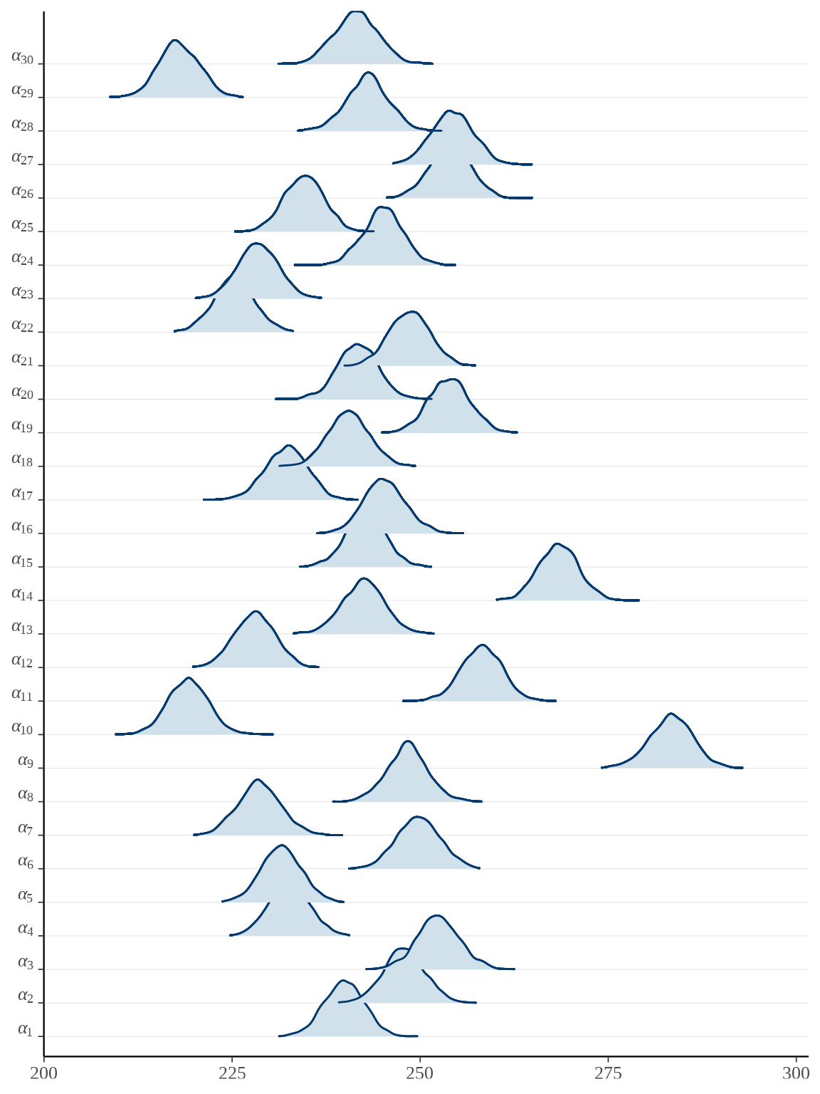
参数向量 \(\boldsymbol{\alpha}\) 的后验估计可以看作 \(x_t = \bar{x}\) 时小鼠的重量,上图即为各个小鼠重量的后验分布。
# plot(rats_fit, pars = "beta", ci_level = 0.8, outer_level = 0.95)
bayesplot::mcmc_areas_ridges(rats_fit, pars = paste0("beta", "[", 1:30, "]")) +
scale_y_discrete(labels = scales::parse_format()) 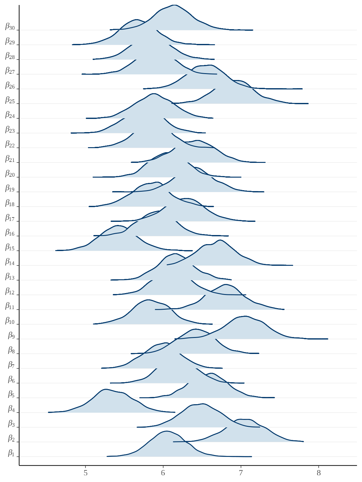
参数向量 \(\boldsymbol{\beta}\) 的后验估计可以看作是小鼠的重量的增长率,上图即为各个小鼠重量的增长率的后验分布。
35.5.2 cmdstanr
从 rstan 包转 cmdstanr 包是非常容易的,只要语法兼容,模型代码可以原封不动。
library(cmdstanr)
mod_rats <- cmdstan_model(
  stan_file = "code/rats.stan",
  compile = TRUE, cpp_options = list(stan_threads = TRUE)
)
fit_rats <- mod_rats$sample(
  data = list(N = N, T = T, y = y, x = x, xbar = xbar), # 数据
  chains = 2,            # 总链条数
  parallel_chains = 2,   # 并行数目
  iter_warmup = 1000,    # 每条链预处理的迭代次数
  iter_sampling = 1000,  # 每条链采样的迭代次数
  threads_per_chain = 2, # 每条链设置 2 个线程
  seed = 20232023,       # 随机数种子
  show_messages = FALSE, # 不显示消息
  adapt_delta = 0.9,     # 接受率
  refresh = 0 # 不显示采样迭代的进度
)
模型输出
# 显示除了参数 alpha 和 beta 以外的结果
vars <- setdiff(fit_rats$metadata()$stan_variables, c("alpha", "beta"))
fit_rats$summary(variables = vars)
#> # A tibble: 10 × 10
#> variable mean median sd mad q5 q95 rhat ess_bulk
#> <chr> <dbl> <dbl> <dbl> <dbl> <dbl> <dbl> <dbl> <dbl>
#> 1 lp__ -438. -438. 6.82 7.26 -450. -427. 1.00 580.
#> 2 alpha_c 243. 243. 2.68 2.53 238. 247. 1.00 2315.
#> 3 beta_c 6.19 6.19 0.106 0.106 6.02 6.36 0.999 3106.
#> 4 tausq_c 37.3 36.8 5.52 5.36 29.2 46.9 1.00 1015.
#> 5 tausq_alp… 215. 206. 61.7 56.2 136. 334. 1.00 2117.
#> 6 tausq_beta 0.271 0.258 0.0941 0.0884 0.145 0.438 1.00 1526.
#> 7 tau_c 6.09 6.06 0.447 0.442 5.40 6.85 1.00 1015.
#> 8 tau_alpha 14.5 14.3 2.03 1.99 11.7 18.3 1.00 2117.
#> 9 tau_beta 0.513 0.508 0.0880 0.0879 0.380 0.662 1.00 1526.
#> 10 alpha0 106. 106. 3.57 3.56 101. 112. 1.00 2843.
#> # ℹ 1 more variable: ess_tail <dbl>诊断信息
35.5.3 brms
brms 包是基于 rstan 包的,基于 Stan 语言做贝叶斯推断,提供与 lme4 包一致的公式语法,且扩展了模型种类。
 Family: gaussian
  Links: mu = identity; sigma = identity
Formula: weight ~ days + (days | rats)
   Data: rats_data (Number of observations: 150)
  Draws: 4 chains, each with iter = 2000; warmup = 1000; thin = 1;
         total post-warmup draws = 4000

Group-Level Effects:
~rats (Number of levels: 30)
                    Estimate Est.Error l-95% CI u-95% CI Rhat Bulk_ESS Tail_ESS
sd(Intercept)          11.27      2.23     7.36    16.08 1.00     2172     2939
sd(days)                0.54      0.09     0.37     0.74 1.00     1380     2356
cor(Intercept,days)    -0.11      0.24    -0.53     0.39 1.00      920     1541

Population-Level Effects:
          Estimate Est.Error l-95% CI u-95% CI Rhat Bulk_ESS Tail_ESS
Intercept   106.47      2.47   101.61   111.23 1.00     2173     2768
days          6.18      0.11     5.96     6.41 1.00     1617     2177

Family Specific Parameters:
      Estimate Est.Error l-95% CI u-95% CI Rhat Bulk_ESS Tail_ESS
sigma     6.15      0.47     5.30     7.14 1.00     1832     3151

Draws were sampled using sampling(NUTS). For each parameter, Bulk_ESS
and Tail_ESS are effective sample size measures, and Rhat is the potential
scale reduction factor on split chains (at convergence, Rhat = 1).
35.5.4 rstanarm
rstanarm 包与 brms 包类似,区别是前者预编译了 Stan 模型,后者根据输入数据和模型编译即时编译,此外,后者支持的模型范围更加广泛。
Model Info:
 function:     stan_lmer
 family:       gaussian [identity]
 formula:      weight ~ days + (days | rats)
 algorithm:    sampling
 sample:       4000 (posterior sample size)
 priors:       see help('prior_summary')
 observations: 150
 groups:       rats (30)

Estimates:
                                      mean    sd      10%     50%     90%
(Intercept)                         106.575   2.236 103.789 106.559 109.415
days                                  6.187   0.111   6.048   6.185   6.329
sigma                                 6.219   0.497   5.626   6.183   6.862
Sigma[rats:(Intercept),(Intercept)] 103.927  42.705  57.329  98.128 159.086
Sigma[rats:days,(Intercept)]         -0.545   1.492  -2.361  -0.402   1.162
Sigma[rats:days,days]                 0.304   0.112   0.181   0.285   0.445

MCMC diagnostics
                                    mcse  Rhat  n_eff
(Intercept)                         0.043 1.000 2753
days                                0.003 1.005 1694
sigma                               0.015 1.001 1172
Sigma[rats:(Intercept),(Intercept)] 1.140 1.000 1403
Sigma[rats:days,(Intercept)]        0.054 1.006  772
Sigma[rats:days,days]               0.003 1.000 1456

For each parameter, mcse is Monte Carlo standard error,
n_eff is a crude measure of effective sample size,
and Rhat is the potential scale reduction factor
on split chains (at convergence Rhat=1).
固定效应的部分,截距和斜率如下:
Estimates:
                                      mean    sd      10%     50%     90%
(Intercept)                         106.575   2.236 103.789 106.559 109.415
days                                  6.187   0.111   6.048   6.185   6.329
模型残差的标准差 sigma、随机效应 Sigma 的随机截距的方差 103.927 、随机斜率的方差 0.304 及其协方差 -0.545。
sigma                                 6.219   0.497   5.626   6.183   6.862
Sigma[rats:(Intercept),(Intercept)] 103.927  42.705  57.329  98.128 159.086
Sigma[rats:days,(Intercept)]         -0.545   1.492  -2.361  -0.402   1.162
Sigma[rats:days,days]                 0.304   0.112   0.181   0.285   0.445
rstanarm 和 brms 包的结果基本一致的。
35.5.5 blme
blme 包 (Chung 等 2013) 基于 lme4 包 (Bates 等 2015) 拟合贝叶斯线性混合效应模型。参考前面 rstan 小节中关于模型参数的先验设置,下面将残差方差的先验设置为逆伽马分布,随机效应的协方差设置为扁平分布。发现拟合结果和 nlme 和 lme4 包的几乎一样。
rats_blme <- blme::blmer(
  weight ~ days + (days | rats), data = rats_data,
  resid.prior = invgamma, cov.prior = NULL
)
summary(rats_blme)
#> Resid prior: invgamma(shape = 0, scale = 0, posterior.scale = var)
#> Prior dev : 7.1328
#>
#> Linear mixed model fit by REML ['blmerMod']
#> Formula: weight ~ days + (days | rats)
#> Data: rats_data
#>
#> REML criterion at convergence: 1095.4
#>
#> Scaled residuals:
#> Min 1Q Median 3Q Max
#> -2.6697 -0.5440 0.1202 0.4968 2.6317
#>
#> Random effects:
#> Groups Name Variance Std.Dev. Corr
#> rats (Intercept) 116.3517 10.7866
#> days 0.2623 0.5121 -0.16
#> Residual 35.3891 5.9489
#> Number of obs: 150, groups: rats, 30
#>
#> Fixed effects:
#> Estimate Std. Error t value
#> (Intercept) 106.5676 2.2977 46.38
#> days 6.1857 0.1056 58.58
#>
#> Correlation of Fixed Effects:
#> (Intr)
#> days -0.343与 lme4 包的函数 lmer() 所不同的是参数 resid.prior 、fixef.prior 和 cov.prior ,它们设置参数的先验分布,其它参数的含义同 lme4 包。resid.prior = invgamma 表示残差方差参数使用逆伽马分布,cov.prior = NULL 表示随机效应的协方差参数使用扁平先验 flat priors。
35.5.6 rjags
rjags (Plummer 2021) 是 JAGS 软件的 R 语言接口,可以拟合分层正态模型,再借助 coda 包 (Plummer 等 2006) 可以分析 JAGS 返回的各项数据。
JAGS 代码和 Stan 代码有不少相似之处,最大的共同点在于以直观的统计模型的符号表示编码模型,仿照 Stan 代码, JAGS 编码的模型(BUGS 代码)如下:
model {
  alpha_c ~ dnorm(0, 1.0E-4);
  beta_c ~ dnorm(0, 1.0E-4);

  tau_c ~ dgamma(0.001, 0.001);
  tau_alpha ~ dgamma(0.001, 0.001);
  tau_beta ~ dgamma(0.001, 0.001);

  sigma_c <- 1.0 / sqrt(tau_c);
  sigma_alpha <- 1.0 / sqrt(tau_alpha);
  sigma_beta <- 1.0 / sqrt(tau_beta);

  for (n in 1:N){
      alpha[n] ~ dnorm(alpha_c, tau_alpha);
      beta[n] ~ dnorm(beta_c, tau_beta);
    for (t in 1:T) {
      y[n,t] ~ dnorm(alpha[n] + beta[n] * (x[t] - xbar), tau_c);
    }
  }
}
转化主要集中在模型块,注意二者概率分布的名称以及参数含义对应关系,JAGS 使用 precision 而不是 standard deviation or variance,比如正态分布中的方差(标准偏差)被替换为其倒数。JAGS 可以省略类型声明(初始化模型时会补上),最后,JAGS 不支持 Stan 中的向量化操作,这种新特性是独特的。
library(rjags)
# 初始值
rats_inits <- list(
  list(".RNG.name" = "base::Marsaglia-Multicarry",
       ".RNG.seed" = 20222022,
       "alpha_c" = 100, "beta_c" = 6, "tau_c" = 5, "tau_alpha" = 10, "tau_beta" = 0.5),
  list(".RNG.name" = "base::Marsaglia-Multicarry",
       ".RNG.seed" = 20232023,
       "alpha_c" = 200, "beta_c" = 10, "tau_c" = 15, "tau_alpha" = 15, "tau_beta" = 1)
)
# 模型
rats_model <- jags.model(
  file = "code/rats.bugs",
  data = list(x = x, y = y, N = 30, T = 5, xbar = 22.0),
  inits = rats_inits,
  n.chains = 2, quiet = TRUE
)
# burn-in
update(rats_model, n.iter = 2000)
# 抽样
rats_samples <- coda.samples(rats_model,
  variable.names = c("alpha_c", "beta_c", "sigma_alpha", "sigma_beta", "sigma_c"),
  n.iter = 4000, thin = 1
)
# 参数的后验估计
summary(rats_samples)
#>
#> Iterations = 2001:6000
#> Thinning interval = 1
#> Number of chains = 2
#> Sample size per chain = 4000
#>
#> 1. Empirical mean and standard deviation for each variable,
#> plus standard error of the mean:
#>
#> Mean SD Naive SE Time-series SE
#> alpha_c 242.4752 2.72749 0.030494 0.031571
#> beta_c 6.1878 0.10798 0.001207 0.001481
#> sigma_alpha 14.6233 2.05688 0.022997 0.025070
#> sigma_beta 0.5176 0.09266 0.001036 0.001741
#> sigma_c 6.0731 0.46425 0.005191 0.007984
#>
#> 2. Quantiles for each variable:
#>
#> 2.5% 25% 50% 75% 97.5%
#> alpha_c 237.0333 240.6832 242.5024 244.2965 247.7816
#> beta_c 5.9785 6.1150 6.1867 6.2593 6.4035
#> sigma_alpha 11.1840 13.1802 14.4152 15.8340 19.2429
#> sigma_beta 0.3571 0.4538 0.5098 0.5734 0.7187
#> sigma_c 5.2384 5.7479 6.0455 6.3803 7.0413输出结果与 rstan 十分一致,且采样速度极快。类似地,alpha0 = alpha_c - xbar * beta_c 可得 alpha0 = 242.4752 - 22 * 6.1878 = 106.3436。
35.5.7 MCMCglmm
同前,先考虑变截距的混合效应模型,MCMCglmm 包 (Hadfield 2010) 给出的拟合结果与 nlme 包很接近。
## 变截距模型
prior1 <- list(
  R = list(V = 1, nu = 0.002),
  G = list(G1 = list(V = 1, nu = 0.002))
)
set.seed(20232023)
rats_mcmc1 <- MCMCglmm::MCMCglmm(
  weight ~ days, random = ~ rats,
  data = rats_data, verbose = FALSE, prior = prior1
)
summary(rats_mcmc1)
#>
#> Iterations = 3001:12991
#> Thinning interval = 10
#> Sample size = 1000
#>
#> DIC: 1088.71
#>
#> G-structure: ~rats
#>
#> post.mean l-95% CI u-95% CI eff.samp
#> rats 213 108.4 336.4 1000
#>
#> R-structure: ~units
#>
#> post.mean l-95% CI u-95% CI eff.samp
#> units 68.58 50.63 86.58 1000
#>
#> Location effects: weight ~ days
#>
#> post.mean l-95% CI u-95% CI eff.samp pMCMC
#> (Intercept) 106.568 100.464 112.897 1000 <0.001 ***
#> days 6.185 6.051 6.315 1000 <0.001 ***
#> ---
#> Signif. codes: 0 '***' 0.001 '**' 0.01 '*' 0.05 '.' 0.1 ' ' 1随机效应的方差(组间方差)为 211.4 ,则标准差为 14.539。残差方差(组内方差)为 68.77,则标准差为 8.293。
再考虑变截距和斜率的混合效应模型。
## 变截距、变斜率模型
prior2 <- list(
  R = list(V = 1, nu = 0.002),
  G = list(G1 = list(V = diag(2), nu = 0.002))
)
set.seed(20232023)
rats_mcmc2 <- MCMCglmm::MCMCglmm(weight ~ days,
  random = ~ us(1 + days):rats,
  data = rats_data, verbose = FALSE, prior = prior2
)
summary(rats_mcmc2)
#>
#> Iterations = 3001:12991
#> Thinning interval = 10
#> Sample size = 1000
#>
#> DIC: 1018.746
#>
#> G-structure: ~us(1 + days):rats
#>
#> post.mean l-95% CI u-95% CI eff.samp
#> (Intercept):(Intercept).rats 124.1327 41.5313 226.059 847.2
#> days:(Intercept).rats -0.7457 -4.3090 2.571 896.6
#> (Intercept):days.rats -0.7457 -4.3090 2.571 896.6
#> days:days.rats 0.2783 0.1067 0.493 786.9
#>
#> R-structure: ~units
#>
#> post.mean l-95% CI u-95% CI eff.samp
#> units 38.14 27.07 51.08 1000
#>
#> Location effects: weight ~ days
#>
#> post.mean l-95% CI u-95% CI eff.samp pMCMC
#> (Intercept) 106.40 101.70 110.78 823.3 <0.001 ***
#> days 6.19 5.99 6.41 963.4 <0.001 ***
#> ---
#> Signif. codes: 0 '***' 0.001 '**' 0.01 '*' 0.05 '.' 0.1 ' ' 1G-structure 代表随机效应部分,R-structure 代表残差效应部分,Location effects 代表固定效应部分。MCMCglmm 包的这套模型表示术语源自商业软件 ASReml 。
随机截距的方差为 124.1327,标准差为 11.1415,随机斜率的方差 0.2783,标准差为 0.5275,随机截距和随机斜率的协方差 -0.7457,相关系数为 -0.1268,这与 nlme 包结果很接近。
35.5.8 INLA
同前,先考虑变截距的混合效应模型。
library(INLA)
inla.setOption(short.summary = TRUE)
# 数值稳定性考虑
rats_data$weight <- rats_data$weight / 400
# 变截距
rats_inla1 <- inla(weight ~ days + f(rats, model = "iid", n = 30),
                  family = "gaussian", data = rats_data)
# 输出结果
summary(rats_inla1)
#> Fixed effects:
#> mean sd 0.025quant 0.5quant 0.975quant mode kld
#> (Intercept) 0.266 0.008 0.252 0.266 0.281 0.266 0
#> days 0.015 0.000 0.015 0.015 0.016 0.015 0
#>
#> Model hyperparameters:
#> mean sd 0.025quant 0.5quant
#> Precision for the Gaussian observations 2414.67 311.30 1852.63 2397.34
#> Precision for rats 888.04 244.24 494.56 859.03
#> 0.975quant mode
#> Precision for the Gaussian observations 3076.07 2367.82
#> Precision for rats 1448.25 806.15
#>
#> is computed再考虑变截距和斜率的混合效应模型。
# https://inla.r-inla-download.org/r-inla.org/doc/latent/iid.pdf
# 二维高斯随机效应的先验为 Wishart prior
rats_data$rats <- as.integer(rats_data$rats)
rats_data$slopeid <- 30 + rats_data$rats
# 变截距、变斜率
rats_inla2 <- inla(
  weight ~ 1 + days + f(rats, model = "iid2d", n = 2 * 30) + f(slopeid, days, copy = "rats"),
  data = rats_data, family = "gaussian"
)
# 输出结果
summary(rats_inla2)
#> Fixed effects:
#> mean sd 0.025quant 0.5quant 0.975quant mode kld
#> (Intercept) 0.266 0.034 0.20 0.266 0.333 0.266 0
#> days 0.015 0.033 -0.05 0.015 0.080 0.015 0
#>
#> Model hyperparameters:
#> mean sd 0.025quant 0.5quant
#> Precision for the Gaussian observations 4522.629 666.547 3334.867 4480.319
#> Precision for rats (component 1) 32.097 7.956 18.938 31.260
#> Precision for rats (component 2) 33.234 8.227 19.603 32.377
#> Rho1:2 for rats -0.001 0.172 -0.335 -0.001
#> 0.975quant mode
#> Precision for the Gaussian observations 5952.954 4407.855
#> Precision for rats (component 1) 50.048 29.770
#> Precision for rats (component 2) 51.773 30.859
#> Rho1:2 for rats 0.334 -0.001
#>
#> is computed
警告
对于变截距和斜率混合效应模型,还未完全弄清楚 INLA 包的输出结果。固定效应部分和残差部分都是和前面一致的,但不清楚随机效应的方差协方差矩阵的估计与 INLA 输出的对应关系。参考《Bayesian inference with INLA》第 3 章第 3 小节。
35.6 总结
基于 rats 数据建立变截距、变斜率的分层正态模型,也是线性混合效应模型的一种特殊情况,下表给出不同方法对模型各个参数的估计及置信区间。
| \(\beta_0\) | \(\beta_1\) | \(\sigma_0\) | \(\sigma_1\) | \(\rho_{\sigma}\) | \(\sigma_{\epsilon}\) | |
|---|---|---|---|---|---|---|
| nlme (REML) | 106.568 | 6.186 | 10.743 | 0.511 | -0.159 | 6.015 |
| lme4 (REML) | 106.568 | 6.186 | 10.744 | 0.511 | -0.16 | 6.015 |
| glmmTMB (REML) | 106.568 | 6.186 | 10.743 | 0.511 | -0.16 | 6.015 |
| MASS (PQL) | 106.568 | 6.186 | 10.495 | 0.500 | -0.15 | 6.015 |
| spaMM (ML) | 106.568 | 6.186 | 10.49 | 0.499 | -0.15 | 6.015 |
| hglm | 106.568 | 6.186 | 10.171 | 0.491 | - | 6.091 |
| mgcv (REML) | 106.568 | 6.186 | 10.311 | 0.492 | - | 6.069 |
表中给出截距 \(\beta_0\) 、斜率 \(\beta_1\) 、随机截距 \(\sigma_0\)、随机斜率 \(\sigma_1\)、随机截距和斜率的相关系数 \(\rho_{\sigma}\)、残差 \(\sigma_{\epsilon}\) 等参数的估计及 95% 的置信区间,四舍五入保留 3 位小数。固定效应部分的结果完全相同,随机效应部分略有不同。
| \(\beta_0\) | \(\beta_1\) | \(\sigma_0\) | \(\sigma_1\) | \(\rho_{\sigma}\) | \(\sigma_{\epsilon}\) | |
|---|---|---|---|---|---|---|
| rstan (NUTS) | 106.4 | 6.2 | 14.6 | 0.5 | - | 6.1 |
| cmdstanr (NUTS) | 106 | 6.19 | 14.5 | 0.513 | - | 6.09 |
| brms (NUTS) | 106.47 | 6.18 | 11.27 | 0.54 | -0.11 | 6.15 |
| rstanarm (NUTS) | 106.575 | 6.187 | 10.194 | 0.551 | -0.0969 | 6.219 |
| blme (REML) | 106.568 | 6.186 | 10.787 | 0.512 | -0.160 | 5.949 |
| rjags (Gibbs) | 106.344 | 6.188 | 14.623 | 0.518 | - | 6.073 |
| MCMCglmm (MCMC) | 106.40 | 6.19 | 11.14 | 0.53 | -0.13 | 6.18 |
其中,INLA 结果的转化未完成,表格中暂缺。rstan 、 cmdstanr 和 rjags 未考虑随机截距和随机斜率的相关性,因此,相关系数暂缺。MCMC 是一种随机优化算法,在不同的实现中,可重复性的要求不同,设置随机数种子仅是其中的一个必要条件,故而,每次运行程序结果可能略微不同,但不影响结论。Stan 相关的 R 包输出结果中,rstan 保留 1 位小数,cmdstanr 保留 3 位有效数字,brms 保留 2 位小数,rstanarm 小数点后保留 3 位有效数字,各不相同,暂未统一处理。
35.7 习题
-
四个组的重复测量数据,如下表所示,建立贝叶斯线性混合效应模型/分层正态模型分析数据,与 nlme 包拟合的结果对比。
表格 35.4: 实验数据 编号 第1组 第2组 第3组 第4组 1 62 63 68 56 2 60 67 66 62 3 63 71 71 60 4 59 64 67 61 5 65 68 63 6 66 68 64 7 63 8 59 \[ \begin{aligned} y_{ij} \sim \mathcal{N}(\theta_i, \sigma^2) &\quad \theta_i \sim \mathcal{N}(\mu, \tau^2) \\ (\mu,\log \sigma, \tau) &\sim \mathrm{uniform\ prior} \\ i = 1,2,3,4 &\quad j = 1,2, \ldots, n_i \end{aligned} \]
\(y_{ij}\) 表示第 \(i\) 组的第 \(j\) 个测量值,\(\theta_i\) 表示第 \(i\) 组的均值,\(\mu\) 表示整体的均值,\(\sigma^2\) 表示组内的方差,\(\tau^2\) 表示组内的方差。
#> Linear mixed-effects model fit by REML #> Data: dat #> AIC BIC logLik #> 121.7804 125.1869 -57.89019 #> #> Random effects: #> Formula: ~1 | group #> (Intercept) Residual #> StdDev: 3.419288 2.366309 #> #> Fixed effects: y ~ 1 #> Value Std.Error DF t-value p-value #> (Intercept) 64.01266 1.780313 20 35.95584 0 #> #> Standardized Within-Group Residuals: #> Min Q1 Med Q3 Max #> -2.18490896 -0.59921167 0.09332131 0.54077636 2.17507789 #> #> Number of Observations: 24 #> Number of Groups: 4随机效应(组间标准差)\(\tau^2\) 3.419288 、残差效应(组内标准差)\(\sigma^2\) 2.366309。截距 \(\mu\) 64.01266 代表整体的均值。各组的均值如下:
也可以调用 rjags 包连接 JAGS 软件做贝叶斯推理,JAGS 代码如下:
model {
  ## specify the distribution for observations
  for(i in 1:n){
    y[i] ~ dnorm(theta[group[i]], 1/sigma2)
  }

  ## specify the prior for theta
  for(j in 1:J){
    theta[j] ~ dnorm(mu, 1/tau2)
  }

  ## specify the prior for hyperparameters
  mu ~ dunif(55, 75)

  log_sigma ~ dunif(-10, 3)
  sigma2 <- exp(2*log_sigma)
  sigma <- exp(log_sigma)

  tau ~ dunif(0, 8)
  tau2 <- pow(tau, 2)
}
完整的运行代码如下:
library(rjags)
# 参考值
mu_a <- min(y)
mu_b <- max(y)
log_sigma_b <- 2 * log(sd(y))
tau_b <- 2 * sd(y)

J <- 4            # 4 个组
n <- length(y)    # 观察值数量
N <- 1500         # 总采样数
nthin <- 1        # 采样间隔
nchains <- 2      # 2 条链
ndiscard <- N / 2 # 预处理阶段 warm-up / burn-in

# 初始值
jags_inits <- list(
  list(".RNG.name" = "base::Marsaglia-Multicarry",
       ".RNG.seed" = 20222022,
       "theta" = rep(3, 4), "mu" = 60, "log_sigma" = 0, "tau" = 1.5),
  list(".RNG.name" = "base::Marsaglia-Multicarry",
       ".RNG.seed" = 20232023,
       "theta" = rep(2, 4), "mu" = 60, "log_sigma" = 1, "tau" = 0.375)
)
# Call JAGS from R
jags_model <- jags.model(
  file = "code/hnm.bugs",
  data = list("y" = y, "group" = group, "J" = J, "n" = n),
  inits = jags_inits, n.chains = nchains, quiet = TRUE
)
# burn-in
update(jags_model, n.iter = ndiscard)
# 抽样
jags_samples <- coda.samples(jags_model,
  variable.names = c('theta','mu','sigma','tau'), n.iter = N
)
# 参数的后验估计
summary(jags_samples)
#> #> Iterations = 1751:3250 #> Thinning interval = 1 #> Number of chains = 2 #> Sample size per chain = 1500 #> #> 1. Empirical mean and standard deviation for each variable, #> plus standard error of the mean: #> #> Mean SD Naive SE Time-series SE #> mu 64.142 2.3470 0.04285 0.05879 #> sigma 2.473 0.4278 0.00781 0.01117 #> tau 4.372 1.5995 0.02920 0.05101 #> theta[1] 61.356 1.2301 0.02246 0.02503 #> theta[2] 65.877 1.0056 0.01836 0.01928 #> theta[3] 67.696 1.0247 0.01871 0.02119 #> theta[4] 61.186 0.8694 0.01587 0.01692 #> #> 2. Quantiles for each variable: #> #> 2.5% 25% 50% 75% 97.5% #> mu 59.145 62.700 64.167 65.510 69.027 #> sigma 1.795 2.165 2.424 2.718 3.471 #> tau 1.846 3.128 4.171 5.464 7.652 #> theta[1] 58.947 60.545 61.342 62.161 63.771 #> theta[2] 63.866 65.228 65.878 66.548 67.872 #> theta[3] 65.665 67.046 67.712 68.337 69.692 #> theta[4] 59.446 60.632 61.189 61.707 62.975 -
基于 lme4 包中学生对老师的评价数据
InstEval建立(广义)线性混合效应模型分析数据。将响应变量(学生评价)视为有序的离散型变量,比较观察两个模型拟合效果(lme4、GLMMadaptive、spaMM 都不支持有序的响应变量,brms 则支持各类有序回归,使用语法与 lme4 完全一样。但是,由于数据规模比较大,计算时间数以天计,可考虑用 Stan 直接编码)。再者,从 Stan 实现的贝叶斯模型来看,感受 Stan 建模的灵活性和扩展性。(nlme 包不支持此等交叉随机效应的表达。)#> 'data.frame': 73421 obs. of 7 variables: #> $ s : Factor w/ 2972 levels "1","2","3","4",..: 1 1 1 1 2 2 3 3 3 3 ... #> $ d : Factor w/ 1128 levels "1","6","7","8",..: 525 560 832 1068 62 406 3 6 19 75 ... #> $ studage: Ord.factor w/ 4 levels "2"<"4"<"6"<"8": 1 1 1 1 1 1 1 1 1 1 ... #> $ lectage: Ord.factor w/ 6 levels "1"<"2"<"3"<"4"<..: 2 1 2 2 1 1 1 1 1 1 ... #> $ service: Factor w/ 2 levels "0","1": 1 2 1 2 1 1 2 1 1 1 ... #> $ dept : Factor w/ 14 levels "15","5","10",..: 14 5 14 12 2 2 13 3 3 3 ... #> $ y : int 5 2 5 3 2 4 4 5 5 4 ...- 因子型变量
s表示 1-2972 位参与评分的学生。 - 因子型变量
d表示 1-2160 位上课的讲师。 - 因子型变量
dept表示课程相关的 1-15 院系。 - 因子型变量
service表示讲师除了授课外,是否承担其它服务。 - 数值型变量
y表示学生给课程的评分,1-5 分对应从坏到很好。
# 数值型的响应变量
fit_lme4 <- lme4::lmer(y ~ 1 + service + (1 | s) + (1 | d) + (1 | dept), data = InstEval)
summary(fit_lme4)
#> Linear mixed model fit by REML ['lmerMod'] #> Formula: y ~ 1 + service + (1 | s) + (1 | d) + (1 | dept) #> Data: InstEval #> #> REML criterion at convergence: 237733.8 #> #> Scaled residuals: #> Min 1Q Median 3Q Max #> -3.0597 -0.7478 0.0404 0.7723 3.1988 #> #> Random effects: #> Groups Name Variance Std.Dev. #> s (Intercept) 0.105998 0.32557 #> d (Intercept) 0.265221 0.51500 #> dept (Intercept) 0.006912 0.08314 #> Residual 1.386500 1.17750 #> Number of obs: 73421, groups: s, 2972; d, 1128; dept, 14 #> #> Fixed effects: #> Estimate Std. Error t value #> (Intercept) 3.28259 0.02935 111.859 #> service1 -0.09264 0.01339 -6.919 #> #> Correlation of Fixed Effects: #> (Intr) #> service1 -0.152lme4 包不支持响应变量为有序分类变量的情形,可用 ordinal 包,此等规模数据,拟合模型需要 5-10 分钟时间。
# 有序因子型的响应变量 InstEval$y <- factor(InstEval$y, ordered = TRUE) library(ordinal) fit_ordinal <- clmm( y ~ 1 + service + (1 | s) + (1 | d) + (1 | dept), data = InstEval, link = "probit", threshold = "equidistant" ) summary(fit_ordinal) ## MCMCglmm library(MCMCglmm) prior2 <- list( R = list(V = 1, nu = 0.002), G = list( G1 = list(V = 1, nu = 0.002), G2 = list(V = 1, nu = 0.002), G3 = list(V = 1, nu = 0.002) ) ) # 响应变量视为数值变量 fit_mcmc2 <- MCMCglmm( y ~ service, random = ~ s + d + dept, family = "gaussian", data = InstEval, verbose = FALSE, prior = prior2 ) # 响应变量视为有序的分类变量 fit_mcmc3 <- MCMCglmm( y ~ service, random = ~ s + d + dept, family = "ordinal", data = InstEval, verbose = FALSE, prior = prior2 )当数据量较大时,MCMCglmm 包拟合模型需要很长时间,放弃,此时,Stan 的相对优势可以体现出来了。Stan 适合大型复杂概率统计模型。
- 因子型变量