21 分类数据的分析
\[ \def\bm#1{{\boldsymbol #1}} \]
- 最常见的两个广义线性模型:泊松和逻辑回归
- 理论公式、R 输出及其解释,应用案例
- 与计数/离散数据的假设检验的关系
- 辛普森悖论,分类数据处理,高维列联表的压缩和分层,边际和条件
- 泰坦尼克号 4x2x2x2 高维复杂列联表分析
计数数据,通俗来说,对象是一个一个或一份一份的,可数的、离散的数据,比如人数。列联表来组织数据,分二维和多维的情况。
21.1 比例检验
21.1.1 单样本检验
比例检验函数 prop.test() 检验比例是否等于给定的值。单样本的比例检验结果中比例的区间估计与 Wilson 区间估计 (Wilson 1927) 是相关的。区间估计与假设检验是有紧密关系的,对于二项分布比例的 11 种区间估计方法的比较 (Newcombe 1998)。
21.1.1.1 近似检验
21.1.1.2 精确检验
函数 binom.test() 来做二项检验,函数 binom.test() 用来检验伯努利试验中成功概率 \(p\) 和给定概率 \(p_0\) 的关系,属于精确检验 (Clopper 和 Pearson 1934)。
比例 \(p\) 的检验,做 \(n\) 次独立试验,样本 \(X_1,\ldots,X_n \sim b(1, p)\),事件发生的总次数 \(\sum_{i=1}^{n}X_i\)。
二项分布中成功概率的检验
#>
#>  Exact binomial test
#>
#> data:  sum(x) and 100
#> number of successes = 23, number of trials = 100, p-value = 5.514e-08
#> alternative hypothesis: true probability of success is not equal to 0.5
#> 95 percent confidence interval:
#>  0.1517316 0.3248587
#> sample estimates:
#> probability of success
#>                   0.23
检验成功概率 p 是否等于 0.5, P 值 \(5.514 \times 10^{-8}\) 结论是拒绝原假设
#>
#>  Exact binomial test
#>
#> data:  sum(x) and 100
#> number of successes = 23, number of trials = 100, p-value = 0.4534
#> alternative hypothesis: true probability of success is not equal to 0.2
#> 95 percent confidence interval:
#>  0.1517316 0.3248587
#> sample estimates:
#> probability of success
#>                   0.23
检验成功概率 p 是否等于 0.2, P 值 0.4534 结论是不能拒绝原假设
切比雪夫不等式(Chebyshev, 1821-1894)。设随机变量 \(X\) 的数学期望和方差都存在,则对任意常数 \(\epsilon > 0\),有
\[ \begin{aligned} P(|X - EX| \geq \epsilon) & \leq \frac{Var(X)}{\epsilon^2} \\ P(|X - EX| \leq \epsilon) & \geq 1 - \frac{Var(X)}{\epsilon^2} \end{aligned} \]
21.1.2 两样本检验
关于两样本的比例检验问题
\[ \begin{aligned} H_0: P_A = P_B \quad vs. \quad H_1: P_A > P_B \\ H_0: P_A = P_B \quad vs. \quad H_1: P_A < P_B \end{aligned} \]
\(H_0\) 成立的情况下,暗示着两个样本来自同一总体。
比例检验函数 prop.test() 用来检验两组或多组二项分布的成功概率(比例)是否相等。
设随机变量 X 服从参数为 \(p\) 的二项分布 \(b(n, p)\), \(Y\) 服从参数为 \(\theta\) 的二项分布 \(b(m,\theta)\), \(m,n\) 都假定为较大的正整数,检验如下问题
\[ H_0: P_A \geq P_B \quad vs. \quad H_1: P_A < P_B \]
根据中心极限定理
\[ \frac{\bar{X} - \bar{Y}}{\sqrt{\frac{p(1-p)}{n} + \frac{\theta(1-\theta)}{m}}} \]
近似服从标准正态分布 \(N(0,1)\)。如果用矩估计 \(\bar{X}\) 和 \(\bar{Y}\) 分别替代总体参数 \(p\) 和 \(\theta\),构造检验统计量
\[ T = \frac{\bar{X} - \bar{Y}}{\sqrt{\frac{\bar{X}(1-\bar{X})}{n} + \frac{\bar{Y}(1-\bar{Y})}{m}}} \]
根据 Slutsky 定理,检验统计量 \(T\) 近似服从标准正态分布,当 \(T\) 偏大时,拒绝 \(H_0\)。该方法的优势在于当 \(n,m\) 比较大时,二项分布比较复杂,无法建立统计表,利用标准正态分布表来给出检验所需要的临界值,简便易行!
当 \(p\) 和 \(\theta\) 都比较小,上述方法检验效果不好,原因在于由中心极限定理对 \(\bar{X}\) 和 \(\bar{Y}\) 的正态分布近似效果不好,或者间接地导致 \(\bar{X}-\bar{Y}\) 的方差偏小,进而 \(T\) 的分辨都不好,而且当 \(p,\theta\) 很接近 1 时,上述现象也会产生!
下面介绍新的解决办法,办法来自两个二项总体成功概率的比较 (宋泽熙 2011)。
上面的检验问题等价于
\[ H_0: \frac{P_A}{P_B} \geq 1 \quad vs. \quad H_1: \frac{P_A}{P_B} < 1 \]
引入检验统计量
\[ T^{\star} = \frac{\bar{X}}{\bar{Y}} \]
同样由 Slutsky 定理和中心极限定理可知, \(\bar{X}/\bar{Y}\) 近似服从 正态分布 \(\mathcal{N}(1,\frac{1-\theta}{m\theta})\)
当 \((T^\star - 1)/\hat\sigma\) 偏大时接受 \(H_0\),临界值可通过 \(\mathcal{N}(0, \hat\sigma^2)\) 分布表计算得到, \(\hat\sigma^2\) 是对 \(\frac{1-\theta}{m\theta}\) 的估计,比如取 \(\hat\sigma^2 = \frac{1-\bar{Y}}{m}\cdot \frac{1}{\bar{Y}}\) 或取 \(\hat\sigma^2 = \frac{1-\bar{Y}}{m}\cdot \frac{1}{\bar{X}}\)
由于渐近方差形如 \(\frac{1-\theta}{m\theta}\),因而在 \(\theta\) 较小,渐近方差较大,克服了之前 \(\bar{X} - \bar{Y}\)的方差较小的问题
\(p,\theta\) 很接近 1 时,我们取检验统计量
\[ T^{\star\star} = \frac{1-\bar{Y}}{1-\bar{X}} \]
结论和 \(T^\star\) 类似,当 \(T^{\star\star}\) 偏大时,拒绝 \(H_0\)。
21.1.3 多样本检验
21.1.3.1 比例齐性检验
对多组数据的比例检验,可以理解为比例齐性检验。
21.1.3.2 比例趋势检验
比例趋势检验函数 prop.trend.test() 的原假设:四个组里面病人中吸烟的比例是相同的。备择假设:四个组的吸烟比例是有趋势的。
\[ \begin{aligned} & H_0: P_1 = P_2 = P_3 = P_4 \\ & H_1: P_1 < P_2 < P_3 < P_4 ~\text{或者}~ P_1 > P_2 > P_3 > P_4 \end{aligned} \]
#>
#>  4-sample test for equality of proportions without continuity correction
#>
#> data:  smokers out of patients
#> X-squared = 12.6, df = 3, p-value = 0.005585
#> alternative hypothesis: two.sided
#> sample estimates:
#>    prop 1    prop 2    prop 3    prop 4
#> 0.9651163 0.9677419 0.9485294 0.8536585#>
#> Chi-squared Test for Trend in Proportions
#>
#> data: smokers out of patients ,
#> using scores: 1 2 3 4
#> X-squared = 8.2249, df = 1, p-value = 0.00413221.2 泊松检验
泊松分布是 1837年由法国数学家泊松 (Poisson, 1781-1840) 首次提出。
\[ p(x) = \frac{\lambda^x\exp(-\lambda)}{x!}, x = 0, 1, \cdots . \]
泊松分布的期望和方差都是 \(\lambda\) ,一般要求 \(\lambda > 0\)。
21.2.1 单样本
poisson.test() 泊松分布的参数 \(\lambda\) 的精确检验,适用于单样本和两样本。
参数 T 数据的时间单位
21.2.2 两样本
21.3 列联表描述
泰坦尼克号乘客生存死亡统计数据,Titanic 数据集
#> , , Age = Child, Survived = No
#>
#>       Sex
#> Class  Male Female
#>   1st     0      0
#>   2nd     0      0
#>   3rd    35     17
#>   Crew    0      0
#>
#> , , Age = Adult, Survived = No
#>
#>       Sex
#> Class  Male Female
#>   1st   118      4
#>   2nd   154     13
#>   3rd   387     89
#>   Crew  670      3
#>
#> , , Age = Child, Survived = Yes
#>
#>       Sex
#> Class  Male Female
#>   1st     5      1
#>   2nd    11     13
#>   3rd    13     14
#>   Crew    0      0
#>
#> , , Age = Adult, Survived = Yes
#>
#>       Sex
#> Class  Male Female
#>   1st    57    140
#>   2nd    14     80
#>   3rd    75     76
#>   Crew  192     20
21.3.1 行列分组表格
代码
| 船舱 | 性别 | 年龄 | 死亡 | 存活 |
|---|---|---|---|---|
| 1st | Male | Child | 0 | 5 |
| 2nd | Male | Child | 0 | 11 |
| 3rd | Male | Child | 35 | 13 |
| Crew | Male | Child | 0 | 0 |
| 1st | Female | Child | 0 | 1 |
| 2nd | Female | Child | 0 | 13 |
| 3rd | Female | Child | 17 | 14 |
| Crew | Female | Child | 0 | 0 |
| 1st | Male | Adult | 118 | 57 |
| 2nd | Male | Adult | 154 | 14 |
| 3rd | Male | Adult | 387 | 75 |
| Crew | Male | Adult | 670 | 192 |
| 1st | Female | Adult | 4 | 140 |
| 2nd | Female | Adult | 13 | 80 |
| 3rd | Female | Adult | 89 | 76 |
| Crew | Female | Adult | 3 | 20 |
21.3.2 百分比堆积图
泰坦尼克号处女航乘客数量按船舱、性别、年龄和存活情况分层, ggstats 包绘制百分比堆积柱形图展示多维分类数据。
代码
library(ggplot2)
library(ggstats)
ggplot(as.data.frame(Titanic)) +
  aes(x = Class, fill = Survived, weight = Freq, by = Class) +
  geom_bar(position = "fill") +
  scale_y_continuous(labels = scales::label_percent()) +
  geom_text(stat = "prop", position = position_fill(.5)) +
  facet_grid(~Sex) +
  labs(x = "船舱", y = "比例", fill = "存活")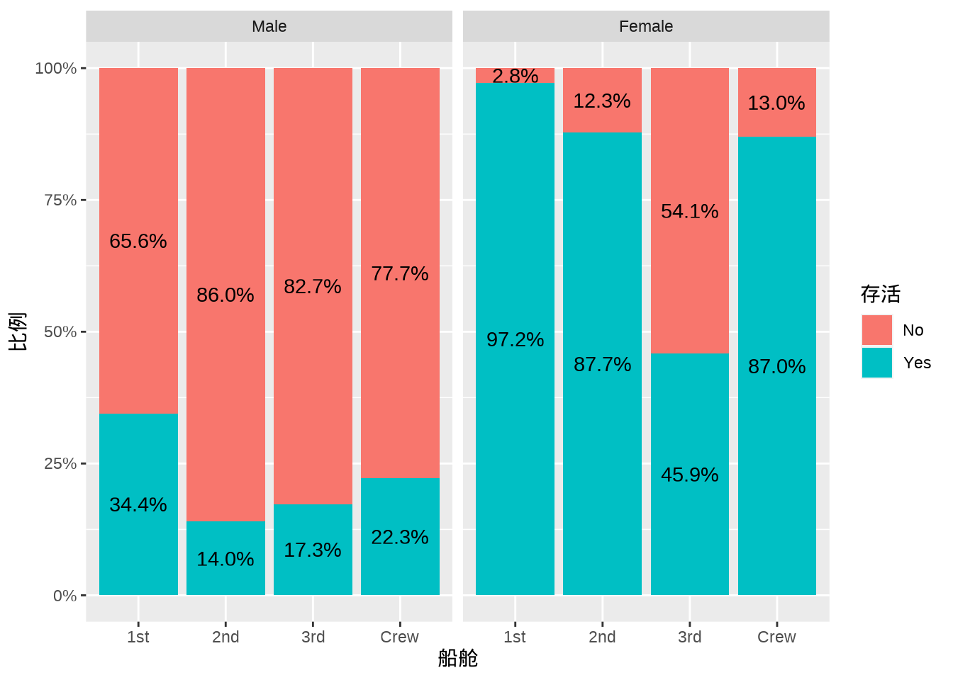
ggstats 包提供的图层 stat_prop() 是 stat_count() 的变种, as.data.frame(Titanic) 中 Age 一列会自动聚合吗? by = Class 按 Class 分组聚合,统计 Survived 的比例,提供 prop 计算的变量,传递给 geom_text() 以添加注释,position 设置将注释放在柱子的中间
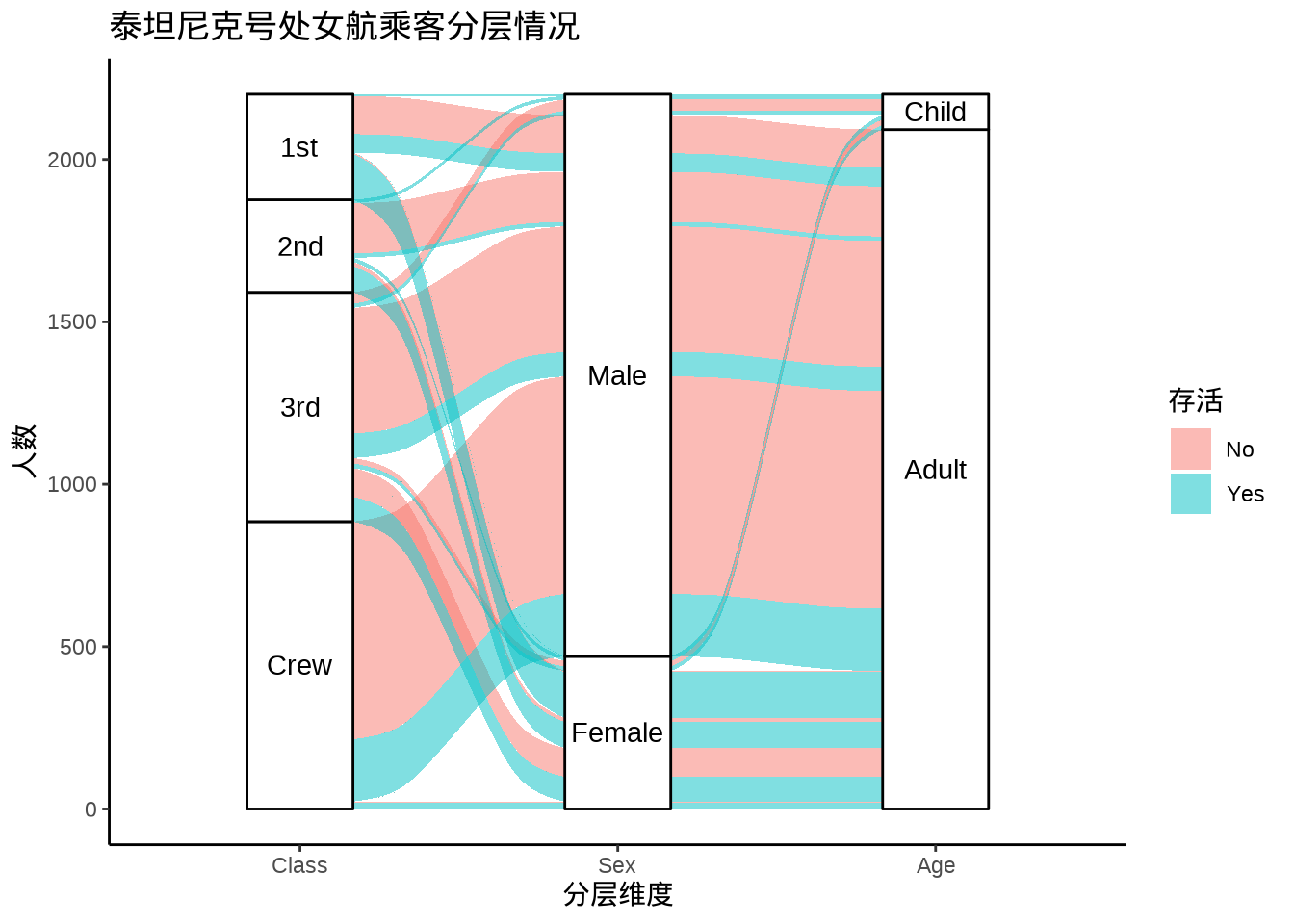
21.3.3 桑基图
用 ggalluvial 包(Brunson 2020)绘制桑基图展示多维分类数据。
代码
library(ggplot2)
library(ggalluvial)
ggplot(
  data = as.data.frame(Titanic),
  aes(axis1 = Class, axis2 = Sex, axis3 = Age, y = Freq)
) +
  scale_x_discrete(limits = c("Class", "Sex", "Age")) +
  geom_alluvium(aes(fill = Survived)) +
  geom_stratum() +
  geom_text(stat = "stratum", aes(label = after_stat(stratum))) +
  theme_classic() +
  labs(
    x = "分层维度", y = "人数", fill = "存活",
    title = "泰坦尼克号处女航乘客分层情况"
  )
21.3.4 马赛克图
代码
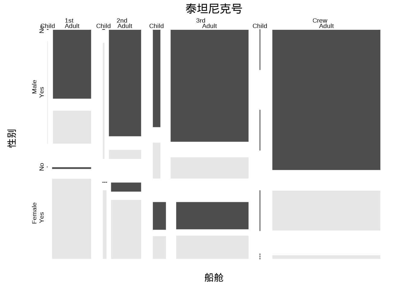
vcd 包针对分类数据做了很多专门的可视化工作,内置了很多数据集和绘图函数,在 Base R 绘图基础上,整合了许多统计分析功能,提供了一个统一的可视化框架(Meyer, Zeileis, 和 Hornik 2006; Zeileis, Meyer, 和 Hornik 2007),更多细节见著作《Discrete Data Analysis with R: Visualization and Modeling Techniques for Categorical and Count Data》及其附带的 R 包 vcdExtra(Friendly 和 Meyer 2016)。
21.4 列联表分析
是否应该按照列联表的维度分类?还是应该从分析的目的和作用出发?比如我的目的是检验独立性。二者似乎也并不冲突。
列联表中的数据服从多项分布,关于独立性检验,有如下几种常见类型:
- 相互独立 Mutual independence 所有变量之间相互独立,\(X \perp Y \perp Z\) 。
- 联合独立 Joint independence 两个变量的联合与第三个变量独立,\(XY \perp Z\) 。
- 边际独立 Marginal independence 当忽略第三个变量时,两个变量是独立的。列联表压缩
- 条件独立 Conditional independence 当固定第三个变量时,两个变量是独立的,\(X \perp Y | Z\)。
本节数据来自著作《An Introduction to Categorical Data Analysis》(Agresti 2007) 的第2章习题 2.33,探索 1976-1977 年美国佛罗里达州的凶杀案件中被告肤色和死刑判决的关系。
代码
tbl <- expand.grid(
  Death = c("Yes", "No"), # 判决结果 是否死刑
  Defend = c("白人", "黑人"),  # 被告 肤色
  Victim = c("白人", "黑人")   # 原告 (被害人)肤色
)
ethnicity <- data.frame(tbl, Freq = c(19, 132, 11, 52, 0, 9,  6, 97))

# 长格式转宽格式
dat1 <- reshape(
  data = ethnicity, direction = "wide",
  idvar = c("Defend", "Victim"),
  timevar = "Death", v.names = "Freq", sep = "_"
)
# 制作表格
gt::gt(dat1) |>
  gt::cols_label(
    Freq_Yes = "是",
    Freq_No = "否",
    Victim = "被害人",
    Defend = "被告"
  ) |>
  gt::tab_spanner(
    label = "死刑",
    columns = c(Freq_Yes, Freq_No)
  ) |>
gt::opt_row_striping()| 被告 | 被害人 | 死刑 | |
|---|---|---|---|
| 是 | 否 | ||
| 白人 | 白人 | 19 | 132 |
| 黑人 | 白人 | 11 | 52 |
| 白人 | 黑人 | 0 | 9 |
| 黑人 | 黑人 | 6 | 97 |
21.4.1 相互独立性
皮尔逊卡方检验( Pearson’s \(\chi^2\) 检验) chisq.test() 常用于列联表独立性检验和方差分析模型的拟合优度检验。下面是一个 \(2 \times 2\) 的列联表。
| 第一列 | 第二列 | 合计 | |
|---|---|---|---|
| 第一行 | \(a\) | \(b\) | \(a+b\) |
| 第二行 | \(c\) | \(d\) | \(c+d\) |
| 合计 | \(a+c\) | \(b+d\) | \(a+b+c+d\) |
#>      Defend
#> Death 白人 黑人
#>   Yes   19   17
#> No 141 149#>
#> Pearson's Chi-squared test with Yates' continuity correction
#>
#> data: m
#> X-squared = 0.086343, df = 1, p-value = 0.7689#>
#> Pearson's Chi-squared test
#>
#> data: m
#> X-squared = 0.22145, df = 1, p-value = 0.6379当被告是白人时,死刑判决 19 个,占总的死刑判决数量的 19/36 = 52.78%,当被告是黑人时,死刑判决 17 个,占总的死刑判决数量的 17/36 = 47.22%。判决结果与被告种族没有显著关系,但与原告(受害人)种族是有关系的,请继续往下看。
# Death 死刑与 Victim (原告)独立性检验
m <- xtabs(Freq ~ Death + Victim, data = ethnicity)
chisq.test(m, correct = TRUE)
#>
#> Pearson's Chi-squared test with Yates' continuity correction
#>
#> data: m
#> X-squared = 4.7678, df = 1, p-value = 0.029#>
#> Pearson's Chi-squared test
#>
#> data: m
#> X-squared = 5.6149, df = 1, p-value = 0.01781当受害人是白人时,死刑判决 30 个,占总的死刑判决数量的 30/36 = 83.33%,当受害人是黑人时,死刑判决 6 个,占总的死刑判决数量的 6/36 = 16.67%。受害人是白人时,死刑判决明显多于黑人。
多维列联表
#> , , Victim = 白人
#>
#>      Defend
#> Death 白人 黑人
#>   Yes   19   11
#>   No   132   52
#>
#> , , Victim = 黑人
#>
#>      Defend
#> Death 白人 黑人
#>   Yes    0    6
#>   No     9   97
判决结果、被告种族、原告种族三者是否存在联合独立性,即考虑 (Victim, Death) 是否与 Defend 独立,(Victim, Defend) 是否与 Death 独立,(Death, Defend) 与 Victim 是否相互独立。
#> $lrt
#> [1] 0.7007504
#>
#> $pearson
#> [1] 0.3751739
#>
#> $df
#> [1] 1
#>
#> $margin
#> $margin[[1]]
#> [1] "Death"  "Defend"
#>
#> $margin[[2]]
#> [1] "Death"  "Victim"
#>
#> $margin[[3]]
#> [1] "Defend" "Victim"似然比检验统计量(Likelihood Ratio Test statistic),皮尔逊 \(\chi^2\) 统计量(Pearson X-square Test statistic)
拟合对数线性模型
模型输出
#>
#> Call:
#> glm(formula = Freq ~ ., family = poisson(link = "log"), data = ethnicity)
#>
#> Coefficients:
#>             Estimate Std. Error z value Pr(>|z|)
#> (Intercept)  2.45087    0.18046  13.582  < 2e-16 ***
#> DeathNo      2.08636    0.17671  11.807  < 2e-16 ***
#> Defend黑人   0.03681    0.11079   0.332     0.74
#> Victim黑人  -0.64748    0.11662  -5.552 2.83e-08 ***
#> ---
#> Signif. codes:  0 '***' 0.001 '**' 0.01 '*' 0.05 '.' 0.1 ' ' 1
#>
#> (Dispersion parameter for poisson family taken to be 1)
#>
#>     Null deviance: 395.92  on 7  degrees of freedom
#> Residual deviance: 137.93  on 4  degrees of freedom
#> AIC: 181.61
#>
#> Number of Fisher Scoring iterations: 5
Pearson \(\chi^2\) 统计量
MASS 包计算模型参数的置信区间
#>                  2.5 %     97.5 %
#> (Intercept)  2.0802598  2.7893934
#> DeathNo      1.7546021  2.4493677
#> Defend黑人  -0.1803969  0.2543149
#> Victim黑人  -0.8790491 -0.4213701
对于单元格总样本量小于 40 或 T 小于 1 时,需采用费希尔精确检验( Fisher ’s Exact 检验)。
21.4.2 边际独立性
费希尔精确检验:固定边际的情况下,检验列联表行和列之间的独立性 fisher.test() 。
fisher.test() 函数用法,统计原理和公式,适用范围和条件,概念背景和历史。
费舍尔 (Sir Ronald Fisher, 1890.2 – 1962.7)1 和一位女士打赌,女士说能品出奶茶中奶和茶的添加顺序。
fisher.test() 针对计数数据,检验列联表中行和列的独立性。
TeaTasting <- matrix(c(3, 1, 1, 3),
  nrow = 2,
  dimnames = list(
    Guess = c("Milk", "Tea"),
    Truth = c("Milk", "Tea")
  )
)
TeaTasting
#> Truth
#> Guess Milk Tea
#> Milk 3 1
#> Tea 1 3#>
#> Fisher's Exact Test for Count Data
#>
#> data: TeaTasting
#> p-value = 0.2429
#> alternative hypothesis: true odds ratio is greater than 1
#> 95 percent confidence interval:
#> 0.3135693 Inf
#> sample estimates:
#> odds ratio
#> 6.408309#>
#> Fisher's Exact Test for Count Data
#>
#> data: TeaTasting
#> p-value = 0.4857
#> alternative hypothesis: true odds ratio is not equal to 1
#> 95 percent confidence interval:
#> 0.2117329 621.9337505
#> sample estimates:
#> odds ratio
#> 6.408309#> [1] 0.242857121.4.3 对称性
用于计数数据的 McNemar 卡方检验( McNemar \(\chi^2\) 检验):检验二维列联表行和列的对称性 mcnemar.test()。怎么理解对称性?其实是配对检验。看帮助实例。
Performance <- matrix(c(794, 86, 150, 570),
  nrow = 2,
  dimnames = list(
    "1st Survey" = c("Approve", "Disapprove"),
    "2nd Survey" = c("Approve", "Disapprove")
  )
)
Performance
#> 2nd Survey
#> 1st Survey Approve Disapprove
#> Approve 794 150
#> Disapprove 86 570#>
#> McNemar's Chi-squared test with continuity correction
#>
#> data: Performance
#> McNemar's chi-squared = 16.818, df = 1, p-value = 4.115e-0521.4.4 条件独立性
用于分层分类数据的 Cochran-Mantel-Haenszel 卡方检验:两个枚举(分类)变量的条件独立性,假定不存在三个因素的交互作用。Cochran-Mantel-Haenszel 检验 mantelhaen.test()
#>  'table' num [1:2, 1:2, 1:6] 512 313 89 19 353 207 17 8 120 205 ...
#>  - attr(*, "dimnames")=List of 3
#>   ..$ Admit : chr [1:2] "Admitted" "Rejected"
#>   ..$ Gender: chr [1:2] "Male" "Female"
#>   ..$ Dept  : chr [1:6] "A" "B" "C" "D" ...
UCBAdmissions 数据集是一个 \(2\times 2 \times 6\) 的三维列联表,R 语言中常用 table 类型表示。实际上,table 类型衍生自 array 数组类型,当把 UCBAdmissions 当作一个数组操作时,1、2、3 分别表示 Admit、Gender、Dept 三个维度。
#>
#>  Mantel-Haenszel chi-squared test with continuity correction
#>
#> data:  UCBAdmissions
#> Mantel-Haenszel X-squared = 1.4269, df = 1, p-value = 0.2323
#> alternative hypothesis: true common odds ratio is not equal to 1
#> 95 percent confidence interval:
#>  0.7719074 1.0603298
#> sample estimates:
#> common odds ratio
#>         0.9046968
没有证据表明院系与性别之间存在关联。在给定院系的情况下,是否录取和性别没有显著关系。
#>         A         B         C         D         E         F
#> 0.3492120 0.8025007 1.1330596 0.9212838 1.2216312 0.8278727
woolf <- function(x) {
x <- x + 1 / 2
k <- dim(x)[3]
or <- apply(x, 3, function(x) (x[1, 1] * x[2, 2]) / (x[1, 2] * x[2, 1]))
w <- apply(x, 3, function(x) 1 / sum(1 / x))
1 - pchisq(sum(w * (log(or) - weighted.mean(log(or), w))^2), k - 1)
}
woolf(UCBAdmissions)#> [1] 0.003427221.5 加州伯克利分校的录取情况
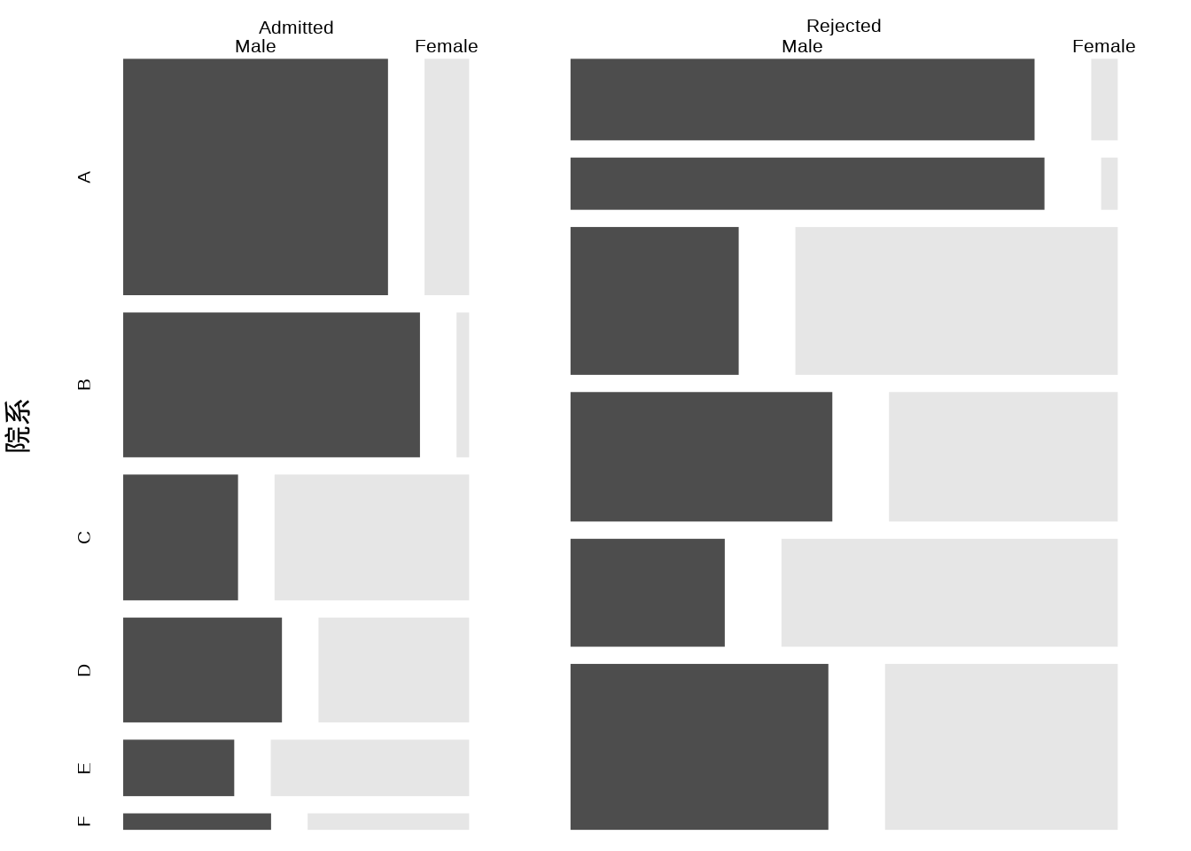
1973 年加州伯克利分校 6 个最大的院系的录取情况见下 表格 21.3 ,研究目标是加州伯克利分校在招生录取工作中是否有性别歧视?
| 院系 | 录取 | 拒绝 | ||
|---|---|---|---|---|
| 男性 | 女性 | 男性 | 女性 | |
| A | 512 | 89 | 313 | 19 |
| B | 353 | 17 | 207 | 8 |
| C | 120 | 202 | 205 | 391 |
| D | 138 | 131 | 279 | 244 |
| E | 53 | 94 | 138 | 299 |
| F | 22 | 24 | 351 | 317 |
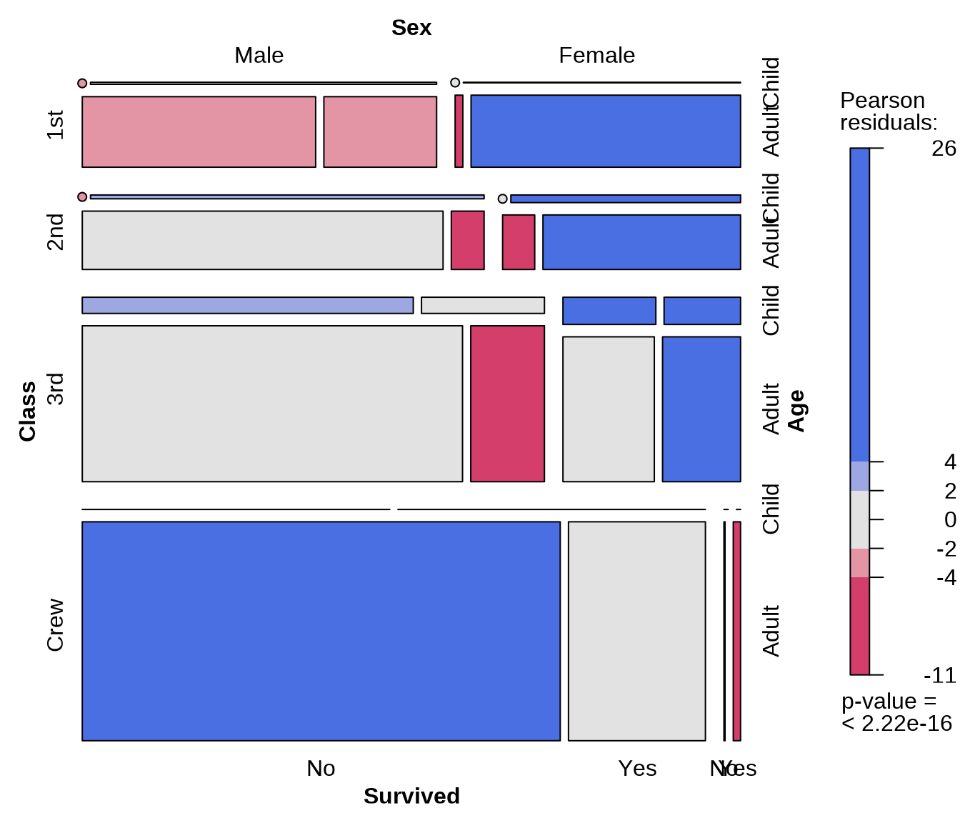
借助马赛克图 图 21.5 可以更加直观的看出数据中的比例关系。
接下来进行定量的分析,首先,按性别和录取情况统计人数,如下:
#>         Admit
#> Gender   Admitted Rejected
#>   Male       1198     1493
#>   Female      557     1278
可以看到,申请加州伯克利分校的女生当中,只有 \(557 / (557 + 1278) = 30.35\%\) 录取了,而男生则有 \(1198 / (1198 + 1493) = 44.52\%\) 的录取率。根据皮尔逊 \(\chi^2\) 检验:
#>
#>  Pearson's Chi-squared test
#>
#> data:  m
#> X-squared = 92.205, df = 1, p-value < 2.2e-16
可知 \(\chi^2\) 统计量的值为 \(92.205\) 且 P 值远远小于 0.05, 差异达到统计显著性,不是随机因素导致的。因此,加州伯克利分校被指控在招生录取工作中存在性别歧视。然而,当我们细分到各个院系去看录取率(录取人数 / 申请人数),结果显示院系 A 的录取率为 64.41%,院系 B 的录取率为 63.24%,依次类推,各院系情况如下:
#>     Admit
#> Dept   Admitted   Rejected
#>    A 0.64415863 0.35584137
#>    B 0.63247863 0.36752137
#>    C 0.35076253 0.64923747
#>    D 0.33964646 0.66035354
#>    E 0.25171233 0.74828767
#>    F 0.06442577 0.93557423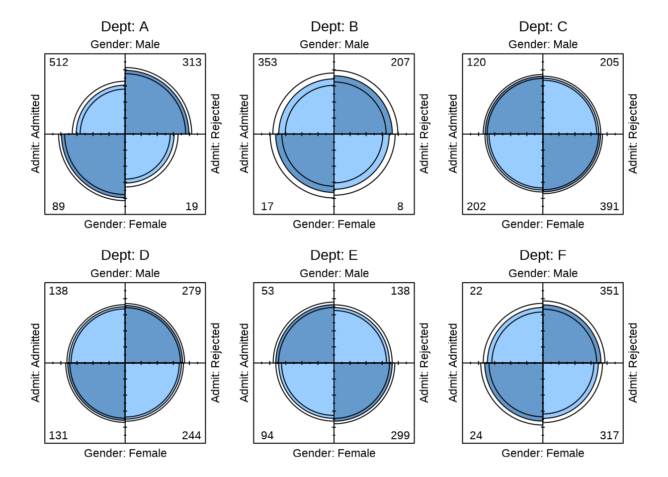
对每个院系,单独使用皮尔逊 \(\chi^2\) 检验,发现只有 A 系的男、女生录取率的差异达到统计显著性,其它系的差异都不显著。辛普森悖论在这里出现了,在分类数据的分析中,常常遇到。
# 以 A 系为例
ma <- xtabs(Freq ~ Gender + Admit,
  subset = Dept == "A",
  data = as.data.frame(UCBAdmissions)
)
chisq.test(ma, correct = FALSE)
#>
#> Pearson's Chi-squared test
#>
#> data: ma
#> X-squared = 17.248, df = 1, p-value = 3.28e-05为了经一步说明此现象的原因,建立对数线性模型来拟合数据,值得一提的是皮尔逊卡方检验可以从对数线性模型的角度来看,而对数线性模型是一种特殊的广义线性模型,针对计数数据建模。
fit_ucb0 <- glm(Freq ~ Dept + Admit + Gender,
  family = poisson(link = "log"),
  data = as.data.frame(UCBAdmissions)
)
summary(fit_ucb0)
#>
#> Call:
#> glm(formula = Freq ~ Dept + Admit + Gender, family = poisson(link = "log"),
#> data = as.data.frame(UCBAdmissions))
#>
#> Coefficients:
#> Estimate Std. Error z value Pr(>|z|)
#> (Intercept) 5.37111 0.03964 135.498 < 2e-16 ***
#> DeptB -0.46679 0.05274 -8.852 < 2e-16 ***
#> DeptC -0.01621 0.04649 -0.349 0.727355
#> DeptD -0.16384 0.04832 -3.391 0.000696 ***
#> DeptE -0.46850 0.05276 -8.879 < 2e-16 ***
#> DeptF -0.26752 0.04972 -5.380 7.44e-08 ***
#> AdmitRejected 0.45674 0.03051 14.972 < 2e-16 ***
#> GenderFemale -0.38287 0.03027 -12.647 < 2e-16 ***
#> ---
#> Signif. codes: 0 '***' 0.001 '**' 0.01 '*' 0.05 '.' 0.1 ' ' 1
#>
#> (Dispersion parameter for poisson family taken to be 1)
#>
#> Null deviance: 2650.1 on 23 degrees of freedom
#> Residual deviance: 2097.7 on 16 degrees of freedom
#> AIC: 2272.7
#>
#> Number of Fisher Scoring iterations: 5添加性别和院系的交互效应后,对数线性模型的 AIC 下降一半多,说明模型的交互效应是显著的,也就是说性别和院系之间存在非常强的关联。
fit_ucb1 <- glm(Freq ~ Dept + Admit + Gender + Dept * Gender,
  family = poisson(link = "log"),
  data = as.data.frame(UCBAdmissions)
)
summary(fit_ucb1)
#>
#> Call:
#> glm(formula = Freq ~ Dept + Admit + Gender + Dept * Gender, family = poisson(link = "log"),
#> data = as.data.frame(UCBAdmissions))
#>
#> Coefficients:
#> Estimate Std. Error z value Pr(>|z|)
#> (Intercept) 5.76801 0.03951 145.992 < 2e-16 ***
#> DeptB -0.38745 0.05475 -7.076 1.48e-12 ***
#> DeptC -0.93156 0.06549 -14.224 < 2e-16 ***
#> DeptD -0.68230 0.06008 -11.356 < 2e-16 ***
#> DeptE -1.46311 0.08030 -18.221 < 2e-16 ***
#> DeptF -0.79380 0.06239 -12.722 < 2e-16 ***
#> AdmitRejected 0.45674 0.03051 14.972 < 2e-16 ***
#> GenderFemale -2.03325 0.10233 -19.870 < 2e-16 ***
#> DeptB:GenderFemale -1.07581 0.22860 -4.706 2.52e-06 ***
#> DeptC:GenderFemale 2.63462 0.12343 21.345 < 2e-16 ***
#> DeptD:GenderFemale 1.92709 0.12464 15.461 < 2e-16 ***
#> DeptE:GenderFemale 2.75479 0.13510 20.391 < 2e-16 ***
#> DeptF:GenderFemale 1.94356 0.12683 15.325 < 2e-16 ***
#> ---
#> Signif. codes: 0 '***' 0.001 '**' 0.01 '*' 0.05 '.' 0.1 ' ' 1
#>
#> (Dispersion parameter for poisson family taken to be 1)
#>
#> Null deviance: 2650.10 on 23 degrees of freedom
#> Residual deviance: 877.06 on 11 degrees of freedom
#> AIC: 1062.1
#>
#> Number of Fisher Scoring iterations: 5此辛普森悖论现象的解释是女生倾向于申请录取率低的院系,而男生倾向于申请录取率高的院系,最终导致整体上,男生的录取率显著高于女生。至于为什么女生会倾向于申请录取率低的院系?这可能要看具体的院系是哪些,招生政策如何?这已经不是仅仅依靠招生办的统计数字就可以完全解释得了的,更多详情见文献 Bickel, Hammel, 和 O’Connell (1975) 。
21.6 分析泰坦尼克号乘客生存率
分析存活率的影响因素。
除了从条件独立性检验的角度,下面从逻辑回归模型的角度分析这个高维列联表数据,由此,我们可以知道假设检验和广义线性模型之间的联系,针对复杂高维列联表数据进行关联分析和解释。
响应变量是乘客的状态,存活还是死亡,titanic_data 是按船舱 Class、性别 Sex 和年龄 Age 分类汇总统计的数据,因此,下面的逻辑回归模型是对乘客群体的建模。
接着,我们查看模型输出的情况
#>
#> Call:
#> glm(formula = cbind(Freq_Yes, Freq_No) ~ Class + Sex + Age, family = binomial(link = "logit"),
#>     data = titanic_data)
#>
#> Coefficients:
#>             Estimate Std. Error z value Pr(>|z|)
#> (Intercept)   0.6853     0.2730   2.510   0.0121 *
#> Class2nd     -1.0181     0.1960  -5.194 2.05e-07 ***
#> Class3rd     -1.7778     0.1716 -10.362  < 2e-16 ***
#> ClassCrew    -0.8577     0.1573  -5.451 5.00e-08 ***
#> SexFemale     2.4201     0.1404  17.236  < 2e-16 ***
#> AgeAdult     -1.0615     0.2440  -4.350 1.36e-05 ***
#> ---
#> Signif. codes:  0 '***' 0.001 '**' 0.01 '*' 0.05 '.' 0.1 ' ' 1
#>
#> (Dispersion parameter for binomial family taken to be 1)
#>
#>     Null deviance: 671.96  on 13  degrees of freedom
#> Residual deviance: 112.57  on  8  degrees of freedom
#> AIC: 171.19
#>
#> Number of Fisher Scoring iterations: 5