36 混合效应模型
\[ \def\bm#1{{\boldsymbol #1}} \]
I think that the formula language does allow expressions with ‘/’ to represent nested factors but I can’t check right now as there is a fire in the building where my office is located. I prefer to simply write nested factors as
factor1 + factor1:factor2.— Douglas Bates 1
混合效应模型在心理学、生态学、计量经济学和空间统计学等领域应用十分广泛。线性混合效应模型有多个化身,比如生态学里的分层线性模型(Hierarchical linear Model,简称 HLM),心理学的多水平线性模型(Multilevel Linear Model)。模型名称的多样性正说明它应用的广泛性! 混合效应模型内容非常多,非常复杂,因此,本章仅对常见的四种类型提供入门级的实战内容。从频率派和贝叶斯派两个角度介绍模型结构及说明、R 代码或 Stan 代码实现及输出结果解释。
除了 R 语言社区提供的开源扩展包,商业的软件有 Mplus 、ASReml 和 SAS 等,而开源的软件 OpenBUGS 、 JAGS 和 Stan 等。混合效应模型的种类非常多,一部分可以在一些流行的 R 包能力范围内解决,其余可以放在更加灵活、扩展性强的框架 Stan 内解决。因此,本章同时介绍 Stan 框架和一些 R 包。
本章用到 4 个数据集,其中 sleepstudy 和 cbpp 均来自 lme4 包 (Bates 等 2015),分别用于介绍线性混合效应模型和广义线性混合效应模型,Loblolly 来自 datasets 包,用于介绍非线性混合效应模型。
在介绍理论的同时给出 R 语言或 S 语言实现的几本参考书籍。
- 《Mixed-Effects Models in S and S-PLUS》(Pinheiro 和 Bates 2000)
- 《Mixed Models: Theory and Applications with R》(Demidenko 2013)
- 《Linear Mixed-Effects Models Using R: A Step-by-Step Approach》(Gałecki 和 Burzykowski 2013)
- 《Linear and Generalized Linear Mixed Models and Their Applications》(Jiang 和 Nguyen 2021)
36.1 线性混合效应模型
I think what we are seeking is the marginal variance-covariance matrix of the parameter estimators (marginal with respect to the random effects random variable, B), which would have the form of the inverse of the crossproduct of a \((q+p)\) by \(p\) matrix composed of the vertical concatenation of \(-L^{-1}RZXRX^{-1}\) and \(RX^{-1}\). (Note: You do not want to calculate the first term by inverting \(L\), use
solve(L, RZX, system = "L")
[…] don’t even think about using
solve(L)don’t!, don’t!, don’t!
have I made myself clear?
don’t do that (and we all know that someone will do exactly that for a very large \(L\) and then send out messages about “R is SOOOOO SLOOOOW!!!!” :-) )
— Douglas Bates 2
- 一般的模型结构和假设
- 一般的模型表达公式
-
nlme 包的函数
lme() - 公式语法和示例模型表示
线性混合效应模型(Linear Mixed Models or Linear Mixed-Effects Models,简称 LME 或 LMM),介绍模型的基础理论,包括一般形式,矩阵表示,参数估计,假设检验,模型诊断,模型评估。参数方法主要是极大似然估计和限制极大似然估计。一般形式如下:
\[ \bm{y} = X\bm{\beta} + Z\bm{u} + \bm{\epsilon} \]
其中,\(\bm{y}\) 是一个向量,代表响应变量,\(X\) 代表固定效应对应的设计矩阵,\(\bm{\beta}\) 是一个参数向量,代表固定效应对应的回归系数,\(Z\) 代表随机效应对应的设计矩阵,\(\bm{u}\) 是一个参数向量,代表随机效应对应的回归系数,\(\bm{\epsilon}\) 表示残差向量。
一般假定随机向量 \(\bm{u}\) 服从多元正态分布,这是无条件分布,随机向量 \(\bm{y}|\bm{u}\) 服从多元正态分布,这是条件分布。
\[ \begin{aligned} \bm{u} &\sim \mathcal{N}(0,\Sigma) \\ \bm{y}|\bm{u} &\sim \mathcal{N}(X\bm{\beta} + Z\bm{u},\sigma^2W) \end{aligned} \]
其中,方差协方差矩阵 \(\Sigma\) 必须是半正定的,\(W\) 是一个对角矩阵。nlme 和 lme4 等 R 包共用一套表示随机效应的公式语法。
sleepstudy 数据集来自 lme4 包,是一个睡眠研究项目的实验数据。实验对象都是有失眠情况的人,有的人有严重的失眠问题(一天只有 3 个小时的睡眠时间)。进入实验后的前10 天的情况,记录平均反应时间、睡眠不足的天数。
#> 'data.frame':    180 obs. of  3 variables:
#>  $ Reaction: num  250 259 251 321 357 ...
#>  $ Days    : num  0 1 2 3 4 5 6 7 8 9 ...
#>  $ Subject : Factor w/ 18 levels "308","309","310",..: 1 1 1 1 1 1 1 1 1 1 ...
Reaction 表示平均反应时间(毫秒),数值型,Days 表示进入实验后的第几天,数值型,Subject 表示参与实验的个体编号,因子型。
#>     Subject
#> Days 308 309 310 330 331 332 333 334 335 337 349 350 351 352 369 370 371 372
#>    0   1   1   1   1   1   1   1   1   1   1   1   1   1   1   1   1   1   1
#>    1   1   1   1   1   1   1   1   1   1   1   1   1   1   1   1   1   1   1
#>    2   1   1   1   1   1   1   1   1   1   1   1   1   1   1   1   1   1   1
#>    3   1   1   1   1   1   1   1   1   1   1   1   1   1   1   1   1   1   1
#>    4   1   1   1   1   1   1   1   1   1   1   1   1   1   1   1   1   1   1
#>    5   1   1   1   1   1   1   1   1   1   1   1   1   1   1   1   1   1   1
#>    6   1   1   1   1   1   1   1   1   1   1   1   1   1   1   1   1   1   1
#>    7   1   1   1   1   1   1   1   1   1   1   1   1   1   1   1   1   1   1
#>    8   1   1   1   1   1   1   1   1   1   1   1   1   1   1   1   1   1   1
#>    9   1   1   1   1   1   1   1   1   1   1   1   1   1   1   1   1   1   1
每个个体每天产生一条数据,下 图 36.1 中每条折线代表一个个体。
library(ggplot2)
ggplot(data = sleepstudy, aes(x = Days, y = Reaction, group = Subject)) +
  geom_line() +
  scale_x_continuous(n.breaks = 6) +
  theme_bw() +
  labs(x = "睡眠不足的天数", y = "平均反应时间")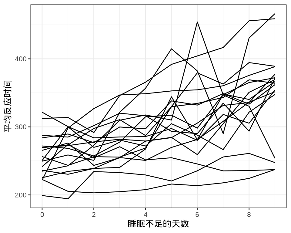
对于连续重复测量的数据(continuous repeated measurement outcomes),也叫纵向数据(longitudinal data),针对不同个体 Subject,相比于上图,下面绘制反应时间 Reaction 随睡眠时间 Days 的变化趋势更合适。图中趋势线是简单线性回归的结果,分面展示不同个体Subject 之间对比。
ggplot(data = sleepstudy, aes(x = Days, y = Reaction)) +
  geom_point() +
  geom_smooth(formula = "y ~ x", method = "lm", se = FALSE) +
  scale_x_continuous(n.breaks = 6) +
  theme_bw() +
  facet_wrap(facets = ~Subject, labeller = "label_both", ncol = 6) +
  labs(x = "睡眠不足的天数", y = "平均反应时间")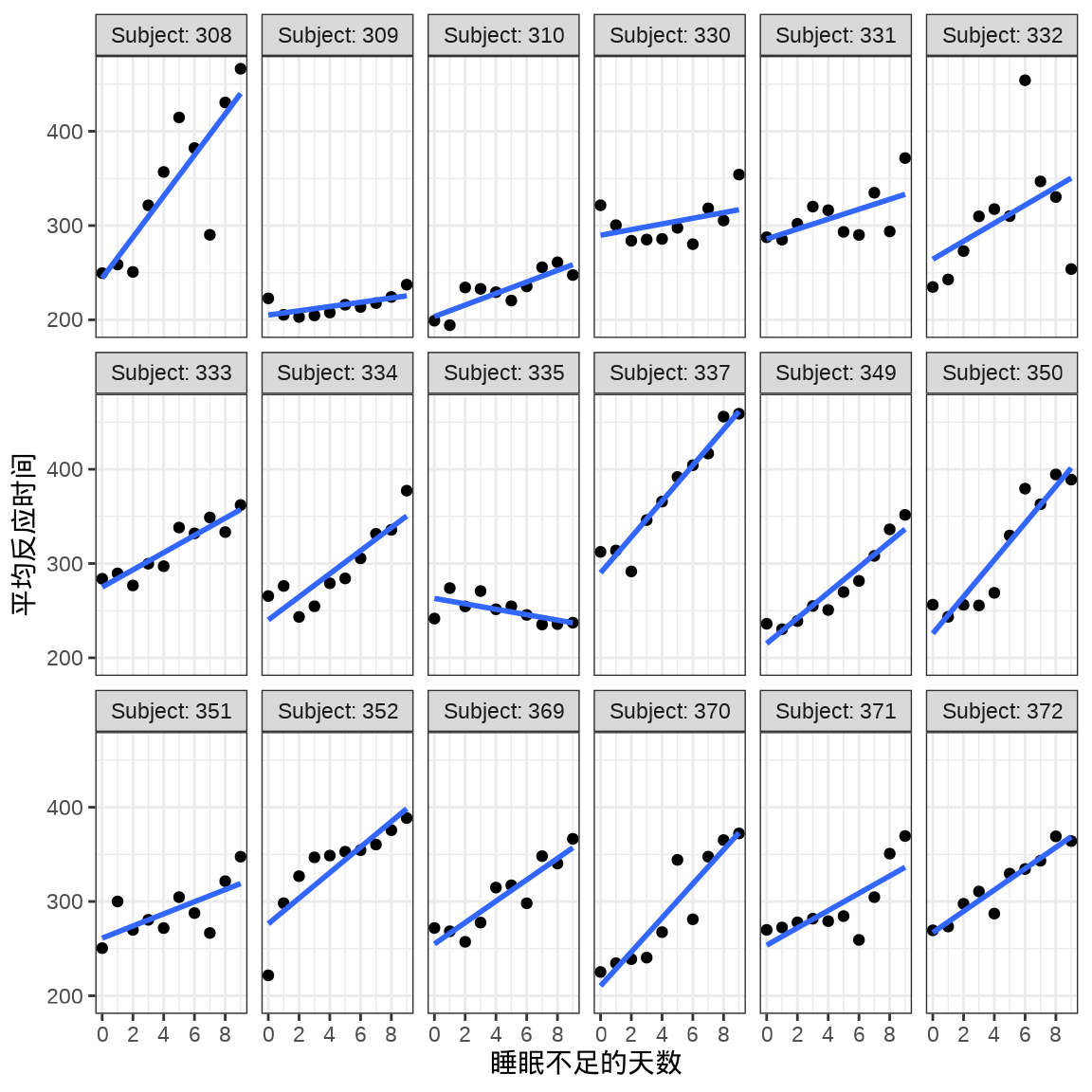
36.1.1 nlme
考虑两水平的混合效应模型,其中随机截距 \(\beta_{0j}\) 和随机斜率 \(\beta_{1j}\),指标 \(j\) 表示分组的编号,也叫变截距和变斜率模型
\[ \begin{aligned} \mathrm{Reaction}_{ij} &= \beta_{0j} + \beta_{1j} \cdot \mathrm{Days}_{ij} + \epsilon_{ij} \\ \beta_{0j} &= \gamma_{00} + U_{0j} \\ \beta_{1j} &= \gamma_{10} + U_{1j} \\ \begin{pmatrix} U_{0j} \\ U_{1j} \end{pmatrix} &\sim \mathcal{N} \begin{bmatrix} \begin{pmatrix} 0 \\ 0 \end{pmatrix} , \begin{pmatrix} \tau^2_{00} & \tau_{01} \\ \tau_{01} & \tau^2_{10} \end{pmatrix} \end{bmatrix} \\ \epsilon_{ij} &\sim \mathcal{N}(0, \sigma^2) \\ i = 0,1,\cdots,9 &\quad j = 308,309,\cdots, 372. \end{aligned} \]
下面用 nlme 包 (Pinheiro 和 Bates 2000) 拟合模型。
library(nlme)
sleep_nlme <- lme(Reaction ~ Days, random = ~ Days | Subject, data = sleepstudy)
summary(sleep_nlme)
#> Linear mixed-effects model fit by REML
#> Data: sleepstudy
#> AIC BIC logLik
#> 1755.628 1774.719 -871.8141
#>
#> Random effects:
#> Formula: ~Days | Subject
#> Structure: General positive-definite, Log-Cholesky parametrization
#> StdDev Corr
#> (Intercept) 24.740241 (Intr)
#> Days 5.922103 0.066
#> Residual 25.591843
#>
#> Fixed effects: Reaction ~ Days
#> Value Std.Error DF t-value p-value
#> (Intercept) 251.40510 6.824516 161 36.83853 0
#> Days 10.46729 1.545783 161 6.77151 0
#> Correlation:
#> (Intr)
#> Days -0.138
#>
#> Standardized Within-Group Residuals:
#> Min Q1 Med Q3 Max
#> -3.95355735 -0.46339976 0.02311783 0.46339621 5.17925089
#>
#> Number of Observations: 180
#> Number of Groups: 18随机效应(Random effects)部分:
#>     (Intercept)       Days
#> 308    2.258754  9.1989366
#> 309  -40.398490 -8.6197167
#> 310  -38.960098 -5.4489048
#> 330   23.690228 -4.8142826
#> 331   22.259981 -3.0698548
#> 332    9.039458 -0.2721585
固定效应(Fixed effects)部分:
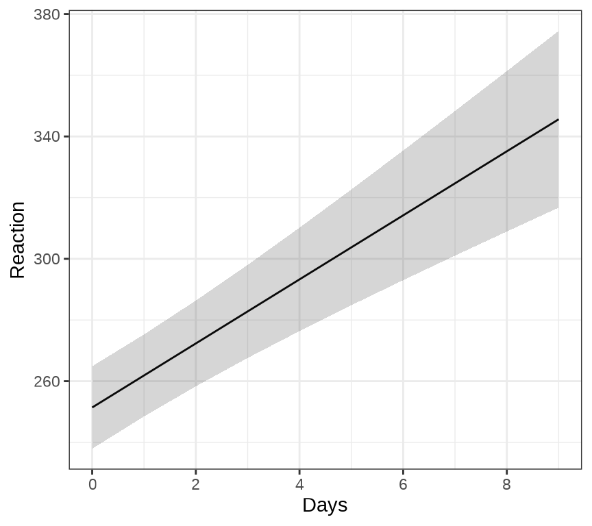
ggeffects 包的函数 ggpredict() 和 ggeffect() 可以用来绘制混合效应模型的边际效应( Marginal Effects),ggPMX 包 可以用来绘制混合效应模型的诊断图。下 图 36.3 展示关于变量 Days 的边际效应图。
36.1.2 MASS
sleep_mass <- MASS::glmmPQL(Reaction ~ Days,
  random = ~ Days | Subject, verbose = FALSE,
  data = sleepstudy, family = gaussian
)
summary(sleep_mass)
#> Linear mixed-effects model fit by maximum likelihood
#> Data: sleepstudy
#> AIC BIC logLik
#> NA NA NA
#>
#> Random effects:
#> Formula: ~Days | Subject
#> Structure: General positive-definite, Log-Cholesky parametrization
#> StdDev Corr
#> (Intercept) 23.780376 (Intr)
#> Days 5.716807 0.081
#> Residual 25.591842
#>
#> Variance function:
#> Structure: fixed weights
#> Formula: ~invwt
#> Fixed effects: Reaction ~ Days
#> Value Std.Error DF t-value p-value
#> (Intercept) 251.40510 6.669396 161 37.69533 0
#> Days 10.46729 1.510647 161 6.92901 0
#> Correlation:
#> (Intr)
#> Days -0.138
#>
#> Standardized Within-Group Residuals:
#> Min Q1 Med Q3 Max
#> -3.94156355 -0.46559311 0.02894656 0.46361051 5.17933587
#>
#> Number of Observations: 180
#> Number of Groups: 1836.1.3 lme4
#> Linear mixed model fit by REML ['lmerMod']
#> Formula: Reaction ~ Days + (Days | Subject)
#>    Data: sleepstudy
#>
#> REML criterion at convergence: 1743.6
#>
#> Scaled residuals:
#>     Min      1Q  Median      3Q     Max
#> -3.9536 -0.4634  0.0231  0.4634  5.1793
#>
#> Random effects:
#>  Groups   Name        Variance Std.Dev. Corr
#>  Subject  (Intercept) 612.10   24.741
#>           Days         35.07    5.922   0.07
#>  Residual             654.94   25.592
#> Number of obs: 180, groups:  Subject, 18
#>
#> Fixed effects:
#>             Estimate Std. Error t value
#> (Intercept)  251.405      6.825  36.838
#> Days          10.467      1.546   6.771
#>
#> Correlation of Fixed Effects:
#>      (Intr)
#> Days -0.138
36.1.4 blme
sleep_blme <- blme::blmer(
  Reaction ~ Days + (Days | Subject), data = sleepstudy,
  control = lme4::lmerControl(check.conv.grad = "ignore"),
  cov.prior = NULL)
summary(sleep_blme)
#> Prior dev : 0
#>
#> Linear mixed model fit by REML ['blmerMod']
#> Formula: Reaction ~ Days + (Days | Subject)
#> Data: sleepstudy
#> Control: lme4::lmerControl(check.conv.grad = "ignore")
#>
#> REML criterion at convergence: 1743.6
#>
#> Scaled residuals:
#> Min 1Q Median 3Q Max
#> -3.9536 -0.4634 0.0231 0.4634 5.1793
#>
#> Random effects:
#> Groups Name Variance Std.Dev. Corr
#> Subject (Intercept) 612.10 24.741
#> Days 35.07 5.922 0.07
#> Residual 654.94 25.592
#> Number of obs: 180, groups: Subject, 18
#>
#> Fixed effects:
#> Estimate Std. Error t value
#> (Intercept) 251.405 6.825 36.838
#> Days 10.467 1.546 6.771
#>
#> Correlation of Fixed Effects:
#> (Intr)
#> Days -0.13836.1.5 brms
 Family: gaussian
  Links: mu = identity; sigma = identity
Formula: Reaction ~ Days + (Days | Subject)
   Data: sleepstudy (Number of observations: 180)
  Draws: 4 chains, each with iter = 2000; warmup = 1000; thin = 1;
         total post-warmup draws = 4000

Group-Level Effects:
~Subject (Number of levels: 18)
                    Estimate Est.Error l-95% CI u-95% CI Rhat Bulk_ESS Tail_ESS
sd(Intercept)          27.03      6.60    15.88    42.13 1.00     1728     2469
sd(Days)                6.61      1.50     4.18     9.97 1.00     1517     2010
cor(Intercept,Days)     0.08      0.29    -0.46     0.65 1.00      991     1521

Population-Level Effects:
          Estimate Est.Error l-95% CI u-95% CI Rhat Bulk_ESS Tail_ESS
Intercept   251.26      7.42   236.27   266.12 1.00     1982     2687
Days         10.36      1.77     6.85    13.85 1.00     1415     1982

Family Specific Parameters:
      Estimate Est.Error l-95% CI u-95% CI Rhat Bulk_ESS Tail_ESS
sigma    25.88      1.54    22.99    29.06 1.00     3204     2869

Draws were sampled using sampling(NUTS). For each parameter, Bulk_ESS
and Tail_ESS are effective sample size measures, and Rhat is the potential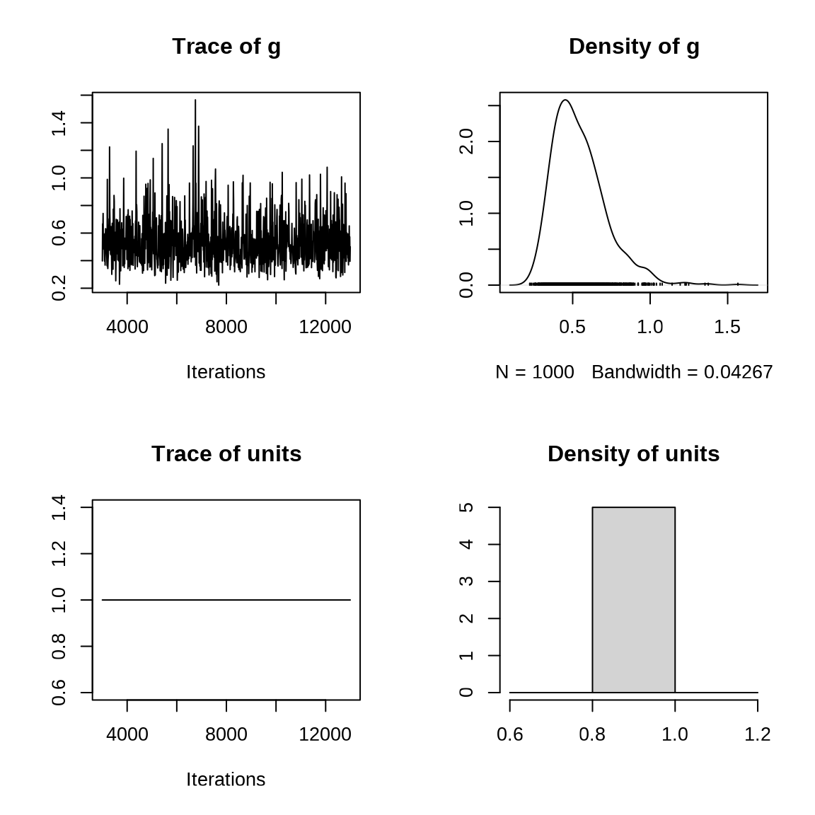
scale reduction factor on split chains (at convergence, Rhat = 1).36.1.6 MCMCglmm
MCMCglmm 包拟合变截距、变斜率模型,随机截距和随机斜率之间存在相关性。
## 变截距、变斜率模型
prior1 <- list(
  R = list(V = 1, fix = 1),
  G = list(G1 = list(V = diag(2), nu = 0.002))
)
set.seed(20232023)
sleep_mcmcglmm <- MCMCglmm::MCMCglmm(
  Reaction ~ Days, random = ~ us(1 + Days):Subject, prior = prior1,
  data = sleepstudy, family = "gaussian", verbose = FALSE
)
summary(sleep_mcmcglmm)
#>
#> Iterations = 3001:12991
#> Thinning interval = 10
#> Sample size = 1000
#>
#> DIC: 94714.46
#>
#> G-structure: ~us(1 + Days):Subject
#>
#> post.mean l-95% CI u-95% CI eff.samp
#> (Intercept):(Intercept).Subject 1005.69 454.97 1840.04 1000.0
#> Days:(Intercept).Subject -34.44 -167.15 84.09 1000.0
#> (Intercept):Days.Subject -34.44 -167.15 84.09 1000.0
#> Days:Days.Subject 52.36 22.74 95.60 902.3
#>
#> R-structure: ~units
#>
#> post.mean l-95% CI u-95% CI eff.samp
#> units 1 1 1 0
#>
#> Location effects: Reaction ~ Days
#>
#> post.mean l-95% CI u-95% CI eff.samp pMCMC
#> (Intercept) 251.374 235.935 265.961 1000 <0.001 ***
#> Days 10.419 7.262 13.976 1000 <0.001 ***
#> ---
#> Signif. codes: 0 '***' 0.001 '**' 0.01 '*' 0.05 '.' 0.1 ' ' 1固定随机效应 R-structure 方差。固定效应 Location effects 截距 (Intercept) 为 251.374,斜率 Days 为 10.419 。
36.1.7 INLA
将数据集 sleepstudy 中的 Reaction 除以 1000,目的是数值稳定性,减小迭代序列的相关性。先考虑变截距模型
library(INLA)
inla.setOption(short.summary = TRUE)
# 做尺度变换
sleepstudy$Reaction <- sleepstudy$Reaction / 1000
# 变截距
sleep_inla1 <- inla(Reaction ~ Days + f(Subject, model = "iid", n = 18),
                  family = "gaussian", data = sleepstudy)
# 输出结果
summary(sleep_inla1)
#> Fixed effects:
#> mean sd 0.025quant 0.5quant 0.975quant mode kld
#> (Intercept) 0.251 0.010 0.232 0.251 0.270 0.251 0
#> Days 0.010 0.001 0.009 0.010 0.012 0.010 0
#>
#> Model hyperparameters:
#> mean sd 0.025quant 0.5quant
#> Precision for the Gaussian observations 1054.07 116.99 840.14 1048.46
#> Precision for Subject 843.97 300.88 391.25 798.36
#> 0.975quant mode
#> Precision for the Gaussian observations 1300.13 1038.99
#> Precision for Subject 1559.54 714.37
#>
#> is computed再考虑变截距和变斜率模型
# https://inla.r-inla-download.org/r-inla.org/doc/latent/iid.pdf
# 二维高斯随机效应的先验为 Wishart prior
sleepstudy$Subject <- as.integer(sleepstudy$Subject)
sleepstudy$slopeid <- 18 + sleepstudy$Subject
# 变截距、变斜率
sleep_inla2 <- inla(
  Reaction ~ 1 + Days + f(Subject, model = "iid2d", n = 2 * 18) + f(slopeid, Days, copy = "Subject"),
  data = sleepstudy, family = "gaussian"
)
# 输出结果
summary(sleep_inla2)
#> Fixed effects:
#> mean sd 0.025quant 0.5quant 0.975quant mode kld
#> (Intercept) 0.251 0.055 0.142 0.251 0.360 0.251 0
#> Days 0.010 0.054 -0.097 0.010 0.118 0.010 0
#>
#> Model hyperparameters:
#> mean sd 0.025quant 0.5quant
#> Precision for the Gaussian observations 1549.519 181.249 1218.046 1540.850
#> Precision for Subject (component 1) 20.871 6.507 10.626 20.024
#> Precision for Subject (component 2) 21.223 6.611 10.803 20.366
#> Rho1:2 for Subject -0.001 0.213 -0.414 -0.002
#> 0.975quant mode
#> Precision for the Gaussian observations 1930.564 1527.270
#> Precision for Subject (component 1) 35.969 18.479
#> Precision for Subject (component 2) 36.552 18.805
#> Rho1:2 for Subject 0.413 -0.003
#>
#> is computed36.2 广义线性混合效应模型
当响应变量分布不再是高斯分布,线性混合效应模型就扩展到广义线性混合效应模型。有一些 R 包可以拟合此类模型,MASS 包的函数 glmmPQL() ,mgcv 包的函数 gam(),lme4 包的函数 glmer() ,GLMMadaptive 包的函数 mixed_model() ,brms 包的函数 brm() 等。
| 响应变量分布 | MASS | mgcv | lme4 | GLMMadaptive | brms |
|---|---|---|---|---|---|
| 伯努利分布 | 支持 | 支持 | 支持 | 支持 | 支持 |
| 二项分布 | 支持 | 支持 | 支持 | 支持 | 支持 |
| 泊松分布 | 支持 | 支持 | 支持 | 支持 | 支持 |
| 负二项分布 | 不支持 | 支持 | 支持 | 支持 | 支持 |
| 伽马分布 | 支持 | 支持 | 支持 | 支持 | 支持 |
函数 glmmPQL() 支持的分布族见函数 glm() 的参数 family ,lme4 包的函数 glmer.nb() 和 GLMMadaptive 包的函数 negative.binomial() 都可用于拟合响应变量服从负二项分布的情况。除了这些常规的分布,GLMMadaptive 和 brms 包还支持许多常见的分布,比如零膨胀的泊松分布、二项分布等,还可以自定义分布。
- 伯努利分布
family = binomial(link = "logit") - 二项分布
family = binomial(link = "logit") - 泊松分布
family = poisson(link = "log") - 负二项分布
lme4::glmer.nb()或GLMMadaptive::negative.binomial() - 伽马分布
family = Gamma(link = "inverse")
GLMMadaptive 包 (Rizopoulos 2023) 的主要函数 mixed_model() 是用来拟合广义线性混合效应模型的。下面以牛传染性胸膜肺炎(Contagious bovine pleuropneumonia,简称 CBPP)数据 cbpp 介绍函数 mixed_model() 的用法,该数据集来自 lme4 包。
#> 'data.frame':    56 obs. of  4 variables:
#>  $ herd     : Factor w/ 15 levels "1","2","3","4",..: 1 1 1 1 2 2 2 3 3 3 ...
#>  $ incidence: num  2 3 4 0 3 1 1 8 2 0 ...
#>  $ size     : num  14 12 9 5 22 18 21 22 16 16 ...
#>  $ period   : Factor w/ 4 levels "1","2","3","4": 1 2 3 4 1 2 3 1 2 3 ...
herd 牛群编号,period 时间段,incidence 感染的数量,size 牛群大小。疾病在种群内扩散
ggplot(data = cbpp, aes(x = herd, y = period)) +
  geom_tile(aes(fill = incidence / size)) +
  scale_fill_viridis_c(label = scales::percent_format(),
                       option = "C", name = "") +
  theme_minimal()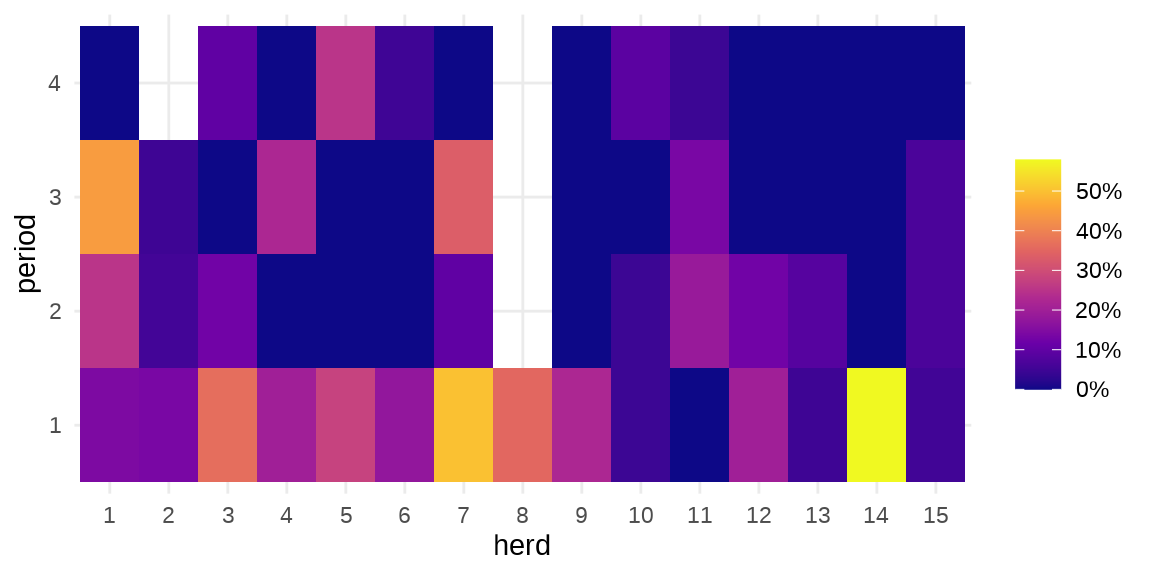
36.2.1 MASS
cbpp_mass <- MASS::glmmPQL(
  cbind(incidence, size - incidence) ~ period,
  random = ~ 1 | herd, verbose = FALSE,
  data = cbpp, family = binomial("logit")
)
summary(cbpp_mass)
#> Linear mixed-effects model fit by maximum likelihood
#> Data: cbpp
#> AIC BIC logLik
#> NA NA NA
#>
#> Random effects:
#> Formula: ~1 | herd
#> (Intercept) Residual
#> StdDev: 0.5563535 1.184527
#>
#> Variance function:
#> Structure: fixed weights
#> Formula: ~invwt
#> Fixed effects: cbind(incidence, size - incidence) ~ period
#> Value Std.Error DF t-value p-value
#> (Intercept) -1.327364 0.2390194 38 -5.553372 0.0000
#> period2 -1.016126 0.3684079 38 -2.758156 0.0089
#> period3 -1.149984 0.3937029 38 -2.920944 0.0058
#> period4 -1.605217 0.5178388 38 -3.099839 0.0036
#> Correlation:
#> (Intr) perid2 perid3
#> period2 -0.399
#> period3 -0.373 0.260
#> period4 -0.282 0.196 0.182
#>
#> Standardized Within-Group Residuals:
#> Min Q1 Med Q3 Max
#> -2.0591168 -0.6493095 -0.2747620 0.5170492 2.6187632
#>
#> Number of Observations: 56
#> Number of Groups: 1536.2.2 GLMMadaptive
library(GLMMadaptive)
cbpp_glmmadaptive <- mixed_model(
  fixed = cbind(incidence, size - incidence) ~ period,
  random = ~ 1 | herd, data = cbpp, family = binomial(link = "logit")
)
summary(cbpp_glmmadaptive)
#>
#> Call:
#> mixed_model(fixed = cbind(incidence, size - incidence) ~ period,
#> random = ~1 | herd, data = cbpp, family = binomial(link = "logit"))
#>
#> Data Descriptives:
#> Number of Observations: 56
#> Number of Groups: 15
#>
#> Model:
#> family: binomial
#> link: logit
#>
#> Fit statistics:
#> log.Lik AIC BIC
#> -91.98337 193.9667 197.507
#>
#> Random effects covariance matrix:
#> StdDev
#> (Intercept) 0.6475934
#>
#> Fixed effects:
#> Estimate Std.Err z-value p-value
#> (Intercept) -1.3995 0.2335 -5.9923 < 1e-04
#> period2 -0.9914 0.3068 -3.2316 0.00123091
#> period3 -1.1278 0.3268 -3.4513 0.00055793
#> period4 -1.5795 0.4276 -3.6937 0.00022101
#>
#> Integration:
#> method: adaptive Gauss-Hermite quadrature rule
#> quadrature points: 11
#>
#> Optimization:
#> method: EM
#> converged: TRUE36.2.3 glmmTMB
cbpp_glmmtmb <- glmmTMB::glmmTMB(
  cbind(incidence, size - incidence) ~ period + (1 | herd),
  data = cbpp, family = binomial, REML = TRUE
)
summary(cbpp_glmmtmb)
#> Family: binomial ( logit )
#> Formula: cbind(incidence, size - incidence) ~ period + (1 | herd)
#> Data: cbpp
#>
#> AIC BIC logLik deviance df.resid
#> 196.4 206.5 -93.2 186.4 55
#>
#> Random effects:
#>
#> Conditional model:
#> Groups Name Variance Std.Dev.
#> herd (Intercept) 0.4649 0.6819
#> Number of obs: 56, groups: herd, 15
#>
#> Conditional model:
#> Estimate Std. Error z value Pr(>|z|)
#> (Intercept) -1.3670 0.2376 -5.752 8.79e-09 ***
#> period2 -0.9693 0.3055 -3.173 0.001509 **
#> period3 -1.1045 0.3255 -3.393 0.000691 ***
#> period4 -1.5519 0.4265 -3.639 0.000274 ***
#> ---
#> Signif. codes: 0 '***' 0.001 '**' 0.01 '*' 0.05 '.' 0.1 ' ' 136.2.4 lme4
cbpp_lme4 <- lme4::glmer(
  cbind(incidence, size - incidence) ~ period + (1 | herd),
  family = binomial("logit"), data = cbpp
)
summary(cbpp_lme4)
#> Generalized linear mixed model fit by maximum likelihood (Laplace
#> Approximation) [glmerMod]
#> Family: binomial ( logit )
#> Formula: cbind(incidence, size - incidence) ~ period + (1 | herd)
#> Data: cbpp
#>
#> AIC BIC logLik deviance df.resid
#> 194.1 204.2 -92.0 184.1 51
#>
#> Scaled residuals:
#> Min 1Q Median 3Q Max
#> -2.3816 -0.7889 -0.2026 0.5142 2.8791
#>
#> Random effects:
#> Groups Name Variance Std.Dev.
#> herd (Intercept) 0.4123 0.6421
#> Number of obs: 56, groups: herd, 15
#>
#> Fixed effects:
#> Estimate Std. Error z value Pr(>|z|)
#> (Intercept) -1.3983 0.2312 -6.048 1.47e-09 ***
#> period2 -0.9919 0.3032 -3.272 0.001068 **
#> period3 -1.1282 0.3228 -3.495 0.000474 ***
#> period4 -1.5797 0.4220 -3.743 0.000182 ***
#> ---
#> Signif. codes: 0 '***' 0.001 '**' 0.01 '*' 0.05 '.' 0.1 ' ' 1
#>
#> Correlation of Fixed Effects:
#> (Intr) perid2 perid3
#> period2 -0.363
#> period3 -0.340 0.280
#> period4 -0.260 0.213 0.19836.2.5 mgcv
或使用 mgcv 包,可以得到近似的结果。随机效应部分可以看作可加的惩罚项
library(mgcv)
cbpp_mgcv <- gam(
  cbind(incidence, size - incidence) ~ period + s(herd, bs = "re"),
  data = cbpp, family = binomial(link = "logit"), method = "REML"
)
summary(cbpp_mgcv)
#>
#> Family: binomial
#> Link function: logit
#>
#> Formula:
#> cbind(incidence, size - incidence) ~ period + s(herd, bs = "re")
#>
#> Parametric coefficients:
#> Estimate Std. Error z value Pr(>|z|)
#> (Intercept) -1.3670 0.2358 -5.799 6.69e-09 ***
#> period2 -0.9693 0.3040 -3.189 0.001428 **
#> period3 -1.1045 0.3241 -3.407 0.000656 ***
#> period4 -1.5519 0.4251 -3.651 0.000261 ***
#> ---
#> Signif. codes: 0 '***' 0.001 '**' 0.01 '*' 0.05 '.' 0.1 ' ' 1
#>
#> Approximate significance of smooth terms:
#> edf Ref.df Chi.sq p-value
#> s(herd) 9.66 14 32.03 3.21e-05 ***
#> ---
#> Signif. codes: 0 '***' 0.001 '**' 0.01 '*' 0.05 '.' 0.1 ' ' 1
#>
#> R-sq.(adj) = 0.515 Deviance explained = 53%
#> -REML = 93.199 Scale est. = 1 n = 56下面给出随机效应的标准差的估计及其上下限,和前面 GLMMadaptive 包和 lme4 包给出的结果也是接近的。
36.2.6 blme
cbpp_blme <- blme::bglmer(
  cbind(incidence, size - incidence) ~ period + (1 | herd),
  family = binomial("logit"), data = cbpp
)
summary(cbpp_blme)
#> Cov prior : herd ~ wishart(df = 3.5, scale = Inf, posterior.scale = cov, common.scale = TRUE)
#> Prior dev : 0.9901
#>
#> Generalized linear mixed model fit by maximum likelihood (Laplace
#> Approximation) [bglmerMod]
#> Family: binomial ( logit )
#> Formula: cbind(incidence, size - incidence) ~ period + (1 | herd)
#> Data: cbpp
#>
#> AIC BIC logLik deviance df.resid
#> 194.2 204.3 -92.1 184.2 51
#>
#> Scaled residuals:
#> Min 1Q Median 3Q Max
#> -2.3670 -0.8121 -0.1704 0.4971 2.7969
#>
#> Random effects:
#> Groups Name Variance Std.Dev.
#> herd (Intercept) 0.5168 0.7189
#> Number of obs: 56, groups: herd, 15
#>
#> Fixed effects:
#> Estimate Std. Error z value Pr(>|z|)
#> (Intercept) -1.4142 0.2466 -5.736 9.7e-09 ***
#> period2 -0.9803 0.3037 -3.227 0.001249 **
#> period3 -1.1171 0.3233 -3.455 0.000549 ***
#> period4 -1.5667 0.4222 -3.710 0.000207 ***
#> ---
#> Signif. codes: 0 '***' 0.001 '**' 0.01 '*' 0.05 '.' 0.1 ' ' 1
#>
#> Correlation of Fixed Effects:
#> (Intr) perid2 perid3
#> period2 -0.342
#> period3 -0.320 0.282
#> period4 -0.246 0.215 0.19936.2.7 brms
表示二项分布,公式语法与前面的 lme4 等包不同。
 Family: binomial
  Links: mu = logit
Formula: incidence | trials(size) ~ period + (1 | herd)
   Data: cbpp (Number of observations: 56)
  Draws: 4 chains, each with iter = 2000; warmup = 1000; thin = 1;
         total post-warmup draws = 4000

Group-Level Effects:
~herd (Number of levels: 15)
              Estimate Est.Error l-95% CI u-95% CI Rhat Bulk_ESS Tail_ESS
sd(Intercept)     0.76      0.22     0.39     1.29 1.00     1483     1962

Population-Level Effects:
          Estimate Est.Error l-95% CI u-95% CI Rhat Bulk_ESS Tail_ESS
Intercept    -1.40      0.26    -1.92    -0.88 1.00     2440     2542
period2      -1.00      0.31    -1.63    -0.41 1.00     5242     2603
period3      -1.14      0.34    -1.83    -0.50 1.00     4938     3481
period4      -1.61      0.44    -2.49    -0.81 1.00     4697     2966

Draws were sampled using sampling(NUTS). For each parameter, Bulk_ESS
and Tail_ESS are effective sample size measures, and Rhat is the potential
scale reduction factor on split chains (at convergence, Rhat = 1).
36.2.8 MCMCglmm
set.seed(20232023)
cbpp_mcmcglmm <- MCMCglmm::MCMCglmm(
  cbind(incidence, size - incidence) ~ period, random = ~herd,
  data = cbpp, family = "multinomial2", verbose = FALSE
)
summary(cbpp_mcmcglmm)
#>
#> Iterations = 3001:12991
#> Thinning interval = 10
#> Sample size = 1000
#>
#> DIC: 538.4141
#>
#> G-structure: ~herd
#>
#> post.mean l-95% CI u-95% CI eff.samp
#> herd 0.0244 1.256e-16 0.1347 186.5
#>
#> R-structure: ~units
#>
#> post.mean l-95% CI u-95% CI eff.samp
#> units 1.098 0.2471 2.158 273.9
#>
#> Location effects: cbind(incidence, size - incidence) ~ period
#>
#> post.mean l-95% CI u-95% CI eff.samp pMCMC
#> (Intercept) -1.5314 -2.1484 -0.8507 1000.0 <0.001 ***
#> period2 -1.2596 -2.2129 -0.1495 854.7 0.006 **
#> period3 -1.3827 -2.3979 -0.2851 691.0 0.012 *
#> period4 -1.9612 -3.3031 -0.7745 572.6 <0.001 ***
#> ---
#> Signif. codes: 0 '***' 0.001 '**' 0.01 '*' 0.05 '.' 0.1 ' ' 1对于服从非高斯分布的响应变量,MCMCglmm 总是假定存在过度离散的情况,即存在一个与分类变量无关的随机变量,或者说存在一个残差服从正态分布的随机变量(效应),可以看作测量误差,这种假定对真实数据建模是有意义的,所以,与以上 MCMCglmm 代码等价的 lme4 包模型代码如下:
cbpp$id <- as.factor(1:dim(cbpp)[1])
cbpp_lme4 <- lme4::glmer(
  cbind(incidence, size - incidence) ~ period + (1 | herd) + (1 | id),
  family = binomial, data = cbpp
)
summary(cbpp_lme4)
#> Generalized linear mixed model fit by maximum likelihood (Laplace
#> Approximation) [glmerMod]
#> Family: binomial ( logit )
#> Formula: cbind(incidence, size - incidence) ~ period + (1 | herd) + (1 |
#> id)
#> Data: cbpp
#>
#> AIC BIC logLik deviance df.resid
#> 186.6 198.8 -87.3 174.6 50
#>
#> Scaled residuals:
#> Min 1Q Median 3Q Max
#> -1.2866 -0.5989 -0.1181 0.3575 1.6216
#>
#> Random effects:
#> Groups Name Variance Std.Dev.
#> id (Intercept) 0.79400 0.8911
#> herd (Intercept) 0.03384 0.1840
#> Number of obs: 56, groups: id, 56; herd, 15
#>
#> Fixed effects:
#> Estimate Std. Error z value Pr(>|z|)
#> (Intercept) -1.5003 0.2967 -5.056 4.27e-07 ***
#> period2 -1.2265 0.4803 -2.554 0.01066 *
#> period3 -1.3288 0.4939 -2.690 0.00713 **
#> period4 -1.8662 0.5936 -3.144 0.00167 **
#> ---
#> Signif. codes: 0 '***' 0.001 '**' 0.01 '*' 0.05 '.' 0.1 ' ' 1
#>
#> Correlation of Fixed Effects:
#> (Intr) perid2 perid3
#> period2 -0.559
#> period3 -0.537 0.373
#> period4 -0.441 0.327 0.314贝叶斯的结果与频率派的结果相近,但还是有明显差异。MCMCglmm 总是假定存在残差,残差的分布服从 0 均值的高斯分布,下面将残差分布的方差固定,重新拟合模型,之后再根据残差方差为 0 调整估计结果。
prior2 <- list(
  R = list(V = 1, fix = 1),
  G = list(G1 = list(V = 1, nu = 0.002))
)
set.seed(20232023)
cbpp_mcmcglmm <- MCMCglmm::MCMCglmm(
  cbind(incidence, size - incidence) ~ period, random = ~herd, prior = prior2,
  data = cbpp, family = "multinomial2", verbose = FALSE
)
summary(cbpp_mcmcglmm)
#>
#> Iterations = 3001:12991
#> Thinning interval = 10
#> Sample size = 1000
#>
#> DIC: 536.3978
#>
#> G-structure: ~herd
#>
#> post.mean l-95% CI u-95% CI eff.samp
#> herd 0.09136 0.0001426 0.4399 312.5
#>
#> R-structure: ~units
#>
#> post.mean l-95% CI u-95% CI eff.samp
#> units 1 1 1 0
#>
#> Location effects: cbind(incidence, size - incidence) ~ period
#>
#> post.mean l-95% CI u-95% CI eff.samp pMCMC
#> (Intercept) -1.5568 -2.1070 -0.8795 841.0 <0.001 ***
#> period2 -1.2424 -2.2081 -0.1868 843.2 0.014 *
#> period3 -1.3416 -2.4066 -0.3783 888.0 0.006 **
#> period4 -1.8745 -3.1598 -0.7545 644.5 <0.001 ***
#> ---
#> Signif. codes: 0 '***' 0.001 '**' 0.01 '*' 0.05 '.' 0.1 ' ' 1下面对结果进行调整
# 调整常数
c2 <- ((16 * sqrt(3)) / (15 * pi))^2
# 固定效应
cbpp_sol_adj <- cbpp_mcmcglmm$Sol / sqrt(1 + c2 * cbpp_mcmcglmm$VCV[, 2])
summary(cbpp_sol_adj)
#>
#> Iterations = 3001:12991
#> Thinning interval = 10
#> Number of chains = 1
#> Sample size per chain = 1000
#>
#> 1. Empirical mean and standard deviation for each variable,
#> plus standard error of the mean:
#>
#> Mean SD Naive SE Time-series SE
#> (Intercept) -1.342 0.2831 0.008953 0.009763
#> period2 -1.071 0.4468 0.014128 0.015386
#> period3 -1.156 0.4603 0.014555 0.015445
#> period4 -1.616 0.5256 0.016621 0.020703
#>
#> 2. Quantiles for each variable:
#>
#> 2.5% 25% 50% 75% 97.5%
#> (Intercept) -1.847 -1.552 -1.347 -1.1431 -0.7918
#> period2 -1.921 -1.352 -1.061 -0.7827 -0.1840
#> period3 -2.066 -1.478 -1.136 -0.8395 -0.3173
#> period4 -2.702 -1.970 -1.608 -1.2584 -0.5811#>
#> Iterations = 3001:12991
#> Thinning interval = 10
#> Number of chains = 1
#> Sample size per chain = 1000
#>
#> 1. Empirical mean and standard deviation for each variable,
#> plus standard error of the mean:
#>
#> Mean SD Naive SE Time-series SE
#> herd 0.06788 0.1335 0.004221 0.00755
#> units 0.74303 0.0000 0.000000 0.00000
#>
#> 2. Quantiles for each variable:
#>
#> 2.5% 25% 50% 75% 97.5%
#> herd 0.0005777 0.004345 0.01809 0.07155 0.4584
#> units 0.7430287 0.743029 0.74303 0.74303 0.7430可以看到,调整后固定效应的部分和前面 lme4 等的输出非常接近,方差成分仍有差距。
36.2.9 INLA
表示二项分布,公式语法与前面的 brms 包和 lme4 等包都不同。
cbpp_inla <- inla(
  formula = incidence ~ period + f(herd, model = "iid", n = 15),
  Ntrials = size, family = "binomial", data = cbpp
)
summary(cbpp_inla)
#> Fixed effects:
#> mean sd 0.025quant 0.5quant 0.975quant mode kld
#> (Intercept) -1.382 0.224 -1.845 -1.375 -0.957 -1.375 0
#> period2 -1.032 0.304 -1.628 -1.032 -0.434 -1.032 0
#> period3 -1.174 0.324 -1.809 -1.174 -0.537 -1.174 0
#> period4 -1.662 0.425 -2.495 -1.662 -0.827 -1.662 0
#>
#> Model hyperparameters:
#> mean sd 0.025quant 0.5quant 0.975quant mode
#> Precision for herd 5.10 6.39 1.02 3.29 18.55 2.17
#>
#> is computed36.3 非线性混合效应模型
Loblolly 数据集来自 R 内置的 datasets 包,记录了 14 颗火炬树种子的生长情况。
| Seed | 3 | 5 | 10 | 15 | 20 | 25 |
|---|---|---|---|---|---|---|
| 301 | 4.51 | 10.89 | 28.72 | 41.74 | 52.70 | 60.92 |
| 303 | 4.55 | 10.92 | 29.07 | 42.83 | 53.88 | 63.39 |
| 305 | 4.79 | 11.37 | 30.21 | 44.40 | 55.82 | 64.10 |
| 307 | 3.91 | 9.48 | 25.66 | 39.07 | 50.78 | 59.07 |
| 309 | 4.81 | 11.20 | 28.66 | 41.66 | 53.31 | 63.05 |
| 311 | 3.88 | 9.40 | 25.99 | 39.55 | 51.46 | 59.64 |
| 315 | 4.32 | 10.43 | 27.16 | 40.85 | 51.33 | 60.07 |
| 319 | 4.57 | 10.57 | 27.90 | 41.13 | 52.43 | 60.69 |
| 321 | 3.77 | 9.03 | 25.45 | 38.98 | 49.76 | 60.28 |
| 323 | 4.33 | 10.79 | 28.97 | 42.44 | 53.17 | 61.62 |
| 325 | 4.38 | 10.48 | 27.93 | 40.20 | 50.06 | 58.49 |
| 327 | 4.12 | 9.92 | 26.54 | 37.82 | 48.43 | 56.81 |
| 329 | 3.93 | 9.34 | 26.08 | 37.79 | 48.31 | 56.43 |
| 331 | 3.46 | 9.05 | 25.85 | 39.15 | 49.12 | 59.49 |
火炬树种子基本决定了树的长势,不同种子预示最后的高度,并且在生长期也是很稳定地生长
ggplot(data = Loblolly, aes(x = age, y = height, color = Seed)) +
  geom_point() +
  geom_line() +
  theme_bw() +
  labs(x = "age (yr)", y = "height (ft)")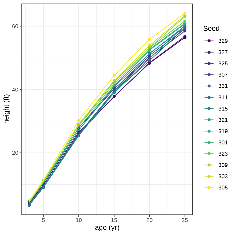
36.3.1 nlme
非线性回归
nfm1 <- nls(height ~ SSasymp(age, Asym, R0, lrc),
           data = Loblolly, subset = Seed == 329)
summary(nfm1)
#>
#> Formula: height ~ SSasymp(age, Asym, R0, lrc)
#>
#> Parameters:
#> Estimate Std. Error t value Pr(>|t|)
#> Asym 94.1282 8.4030 11.202 0.001525 **
#> R0 -8.2508 1.2261 -6.729 0.006700 **
#> lrc -3.2176 0.1386 -23.218 0.000175 ***
#> ---
#> Signif. codes: 0 '***' 0.001 '**' 0.01 '*' 0.05 '.' 0.1 ' ' 1
#>
#> Residual standard error: 0.7493 on 3 degrees of freedom
#>
#> Number of iterations to convergence: 0
#> Achieved convergence tolerance: 3.919e-07非线性函数 SSasymp() 的内容如下
\[ \mathrm{Asym}+(\mathrm{R0}-\mathrm{Asym})\times\exp\big(-\exp(\mathrm{lrc})\times\mathrm{input}\big) \]
其中,\(\mathrm{Asym}\) 、\(\mathrm{R0}\) 、\(\mathrm{lrc}\) 是参数,\(\mathrm{input}\) 是输入值。
示例来自 nlme 包的函数 nlme() 帮助文档
nfm2 <- nlme(height ~ SSasymp(age, Asym, R0, lrc),
  data = Loblolly,
  fixed = Asym + R0 + lrc ~ 1,
  random = Asym ~ 1,
  start = c(Asym = 103, R0 = -8.5, lrc = -3.3)
)
summary(nfm2)
#> Nonlinear mixed-effects model fit by maximum likelihood
#> Model: height ~ SSasymp(age, Asym, R0, lrc)
#> Data: Loblolly
#> AIC BIC logLik
#> 239.4856 251.6397 -114.7428
#>
#> Random effects:
#> Formula: Asym ~ 1 | Seed
#> Asym Residual
#> StdDev: 3.650642 0.7188625
#>
#> Fixed effects: Asym + R0 + lrc ~ 1
#> Value Std.Error DF t-value p-value
#> Asym 101.44960 2.4616951 68 41.21128 0
#> R0 -8.62733 0.3179505 68 -27.13420 0
#> lrc -3.23375 0.0342702 68 -94.36052 0
#> Correlation:
#> Asym R0
#> R0 0.704
#> lrc -0.908 -0.827
#>
#> Standardized Within-Group Residuals:
#> Min Q1 Med Q3 Max
#> -2.23601930 -0.62380854 0.05917466 0.65727206 1.95794425
#>
#> Number of Observations: 84
#> Number of Groups: 14#> Nonlinear mixed-effects model fit by maximum likelihood
#> Model: height ~ SSasymp(age, Asym, R0, lrc)
#> Data: Loblolly
#> AIC BIC logLik
#> 238.9662 253.5511 -113.4831
#>
#> Random effects:
#> Formula: list(Asym ~ 1, lrc ~ 1)
#> Level: Seed
#> Structure: Diagonal
#> Asym lrc Residual
#> StdDev: 2.806185 0.03449969 0.6920003
#>
#> Fixed effects: Asym + R0 + lrc ~ 1
#> Value Std.Error DF t-value p-value
#> Asym 101.85205 2.3239828 68 43.82651 0
#> R0 -8.59039 0.3058441 68 -28.08747 0
#> lrc -3.24011 0.0345017 68 -93.91167 0
#> Correlation:
#> Asym R0
#> R0 0.727
#> lrc -0.902 -0.796
#>
#> Standardized Within-Group Residuals:
#> Min Q1 Med Q3 Max
#> -2.06072906 -0.69785679 0.08721706 0.73687722 1.79015782
#>
#> Number of Observations: 84
#> Number of Groups: 1436.3.2 lme4
lme4 的公式语法是与 nlme 包不同的。
lob_lme4 <- lme4::nlmer(
  height ~ SSasymp(age, Asym, R0, lrc) ~ (Asym + R0 + lrc) + (Asym | Seed),
  data = Loblolly,
  start = c(Asym = 103, R0 = -8.5, lrc = -3.3)
)
summary(lob_lme4)
#> Nonlinear mixed model fit by maximum likelihood ['nlmerMod']
#> Formula: height ~ SSasymp(age, Asym, R0, lrc) ~ (Asym + R0 + lrc) + (Asym |
#> Seed)
#> Data: Loblolly
#>
#> AIC BIC logLik deviance df.resid
#> 239.4 251.5 -114.7 229.4 79
#>
#> Scaled residuals:
#> Min 1Q Median 3Q Max
#> -2.24149 -0.62546 0.08326 0.67711 1.91351
#>
#> Random effects:
#> Groups Name Variance Std.Dev.
#> Seed Asym 13.5121 3.6759
#> Residual 0.5161 0.7184
#> Number of obs: 84, groups: Seed, 14
#>
#> Fixed effects:
#> Estimate Std. Error t value
#> Asym 102.119832 0.012378 8249.9
#> R0 -8.549401 0.012354 -692.0
#> lrc -3.243973 0.008208 -395.2
#>
#> Correlation of Fixed Effects:
#> Asym R0
#> R0 0.000
#> lrc -0.008 -0.03436.3.3 brms
根据数据的情况,设定参数的先验分布
根据模型表达式编码
 Family: gaussian
  Links: mu = identity; sigma = identity
Formula: height ~ Asym + (R0 - Asym) * exp(-exp(lrc) * age)
         R0 ~ 1
         lrc ~ 1
         Asym ~ 1 + (1 | Seed)
   Data: Loblolly (Number of observations: 84)
  Draws: 4 chains, each with iter = 2000; warmup = 1000; thin = 1;
         total post-warmup draws = 4000

Group-Level Effects:
~Seed (Number of levels: 14)
                   Estimate Est.Error l-95% CI u-95% CI Rhat Bulk_ESS Tail_ESS
sd(Asym_Intercept)     3.90      1.09     2.24     6.51 1.00     1033     1647

Population-Level Effects:
               Estimate Est.Error l-95% CI u-95% CI Rhat Bulk_ESS Tail_ESS
R0_Intercept      -8.53      0.43    -9.37    -7.68 1.00     2236     1434
lrc_Intercept     -3.23      0.02    -3.27    -3.20 1.00      981     1546
Asym_Intercept   101.00      0.10   100.80   101.20 1.00     4443     2907

Family Specific Parameters:
      Estimate Est.Error l-95% CI u-95% CI Rhat Bulk_ESS Tail_ESS
sigma     1.68      0.25     1.20     2.17 1.00     1910     2258

Draws were sampled using sampling(NUTS). For each parameter, Bulk_ESS
and Tail_ESS are effective sample size measures, and Rhat is the potential
scale reduction factor on split chains (at convergence, Rhat = 1).
36.4 模拟实验比较(补充)
从广义线性混合效应模型生成模拟数据,用至少 6 个不同的 R 包估计模型参数,比较和归纳不同估计方法和实现算法的效果。举例:带漂移项的泊松型广义线性混合效应模型。\(y_{ij}\) 表示响应变量,\(\bm{u}\) 表示随机效应,\(o_{ij}\) 表示漂移项。
\[ \begin{aligned} y_{ij}|\bm{u} &\sim \mathrm{Poisson}(o_{ij}\lambda_{ij}) \\ \log(\lambda_{ij}) &= \beta_{ij}x_{ij} + u_{j} \\ u_j &\sim \mathcal{N}(0, \sigma^2) \\ i = 1,2,\ldots, n &\quad j = 1,2,\ldots,q \end{aligned} \]
首先准备数据
set.seed(2023)
Ngroups <- 25 # 一个随机效应分 25 个组
NperGroup <- 100 # 每个组 100 个观察值
# 样本量
N <- Ngroups * NperGroup
# 截距和两个协变量的系数
beta <- c(0.5, 0.3, 0.2)
# 两个协变量
X <- MASS::mvrnorm(N, mu = rep(0, 2), Sigma = matrix(c(1, 0.8, 0.8, 1), 2))
# 漂移项
o <- rep(c(2, 4), each = N / 2)
# 分 25 个组 每个组 100 个观察值
g <- factor(rep(1:Ngroups, each = NperGroup))
u <- rnorm(Ngroups, sd = .5) # 随机效应的标准差 0.5
# 泊松分布的期望
lambda <- o * exp(cbind(1, X) %*% beta + u[g])
# 响应变量的值
y <- rpois(N, lambda = lambda)
# 模拟的数据集
sim_data <- data.frame(y, X, o, g)
colnames(sim_data) <- c("y", "x1", "x2", "o", "g")
36.4.1 lme4
# 模型拟合
fit_lme4 <- lme4::glmer(y ~ x1 + x2 + (1 | g),
  data = sim_data, offset = log(o), family = poisson(link = "log")
)
summary(fit_lme4)
#> Generalized linear mixed model fit by maximum likelihood (Laplace
#> Approximation) [glmerMod]
#> Family: poisson ( log )
#> Formula: y ~ x1 + x2 + (1 | g)
#> Data: sim_data
#> Offset: log(o)
#>
#> AIC BIC logLik deviance df.resid
#> 11065.6 11088.9 -5528.8 11057.6 2496
#>
#> Scaled residuals:
#> Min 1Q Median 3Q Max
#> -3.0650 -0.7177 -0.0827 0.6334 4.0103
#>
#> Random effects:
#> Groups Name Variance Std.Dev.
#> g (Intercept) 0.4074 0.6383
#> Number of obs: 2500, groups: g, 25
#>
#> Fixed effects:
#> Estimate Std. Error z value Pr(>|z|)
#> (Intercept) 0.55607 0.12805 4.343 1.41e-05 ***
#> x1 0.28442 0.01280 22.214 < 2e-16 ***
#> x2 0.20851 0.01294 16.117 < 2e-16 ***
#> ---
#> Signif. codes: 0 '***' 0.001 '**' 0.01 '*' 0.05 '.' 0.1 ' ' 1
#>
#> Correlation of Fixed Effects:
#> (Intr) x1
#> x1 -0.008
#> x2 -0.008 -0.82136.4.2 GLMMadaptive
对随机效应采用 adaptive Gauss-Hermite quadrature 积分
library(GLMMadaptive)
fit_glmmadaptive <- mixed_model(
  fixed = y ~ x1 + x2 + offset(log(o)),
  random = ~ 1 | g, data = sim_data,
  family = poisson(link = "log")
)
summary(fit_glmmadaptive)
#>
#> Call:
#> mixed_model(fixed = y ~ x1 + x2 + offset(log(o)), random = ~1 |
#> g, data = sim_data, family = poisson(link = "log"))
#>
#> Data Descriptives:
#> Number of Observations: 2500
#> Number of Groups: 25
#>
#> Model:
#> family: poisson
#> link: log
#>
#> Fit statistics:
#> log.Lik AIC BIC
#> -5528.78 11065.56 11070.44
#>
#> Random effects covariance matrix:
#> StdDev
#> (Intercept) 0.6417329
#>
#> Fixed effects:
#> Estimate Std.Err z-value p-value
#> (Intercept) 0.5647 0.1288 4.3863 < 1e-04
#> x1 0.2844 0.0128 22.2059 < 1e-04
#> x2 0.2085 0.0129 16.1096 < 1e-04
#>
#> Integration:
#> method: adaptive Gauss-Hermite quadrature rule
#> quadrature points: 11
#>
#> Optimization:
#> method: hybrid EM and quasi-Newton
#> converged: TRUE36.4.3 glmmTMB
fit_glmmtmb <- glmmTMB::glmmTMB(
  y ~ x1 + x2 + (1 | g), offset = log(o),
  data = sim_data, family = poisson, REML = TRUE
)
summary(fit_glmmtmb)
#> Family: poisson ( log )
#> Formula: y ~ x1 + x2 + (1 | g)
#> Data: sim_data
#> Offset: log(o)
#>
#> AIC BIC logLik deviance df.resid
#> 11082.7 11106.0 -5537.3 11074.7 2499
#>
#> Random effects:
#>
#> Conditional model:
#> Groups Name Variance Std.Dev.
#> g (Intercept) 0.4245 0.6515
#> Number of obs: 2500, groups: g, 25
#>
#> Conditional model:
#> Estimate Std. Error z value Pr(>|z|)
#> (Intercept) 0.55710 0.13069 4.263 2.02e-05 ***
#> x1 0.28442 0.01281 22.206 < 2e-16 ***
#> x2 0.20851 0.01294 16.111 < 2e-16 ***
#> ---
#> Signif. codes: 0 '***' 0.001 '**' 0.01 '*' 0.05 '.' 0.1 ' ' 136.4.4 hglm
hglm 包的名称是 Hierarchical Generalized Linear Models 的首字母缩写拼成的。
# extended quasi likelihood (EQL) method
fit_hglm <- hglm::hglm(
  fixed =  y ~ x1 + x2, random = ~ 1 | g,
  family = poisson(link = "log"),
  offset = log(o), data = sim_data
)
summary(fit_hglm)
#> Call:
#> hglm.formula(family = poisson(link = "log"), fixed = y ~ x1 +
#> x2, random = ~1 | g, data = sim_data, offset = log(o))
#>
#> ----------
#> MEAN MODEL
#> ----------
#>
#> Summary of the fixed effects estimates:
#>
#> Estimate Std. Error t-value Pr(>|t|)
#> (Intercept) 0.55720 0.13058 4.267 2.05e-05 ***
#> x1 0.28442 0.01316 21.609 < 2e-16 ***
#> x2 0.20851 0.01330 15.678 < 2e-16 ***
#> ---
#> Signif. codes: 0 '***' 0.001 '**' 0.01 '*' 0.05 '.' 0.1 ' ' 1
#> Note: P-values are based on 2473 degrees of freedom
#>
#> Summary of the random effects estimates:
#>
#> Estimate Std. Error
#> g1 0.6643 0.1352
#> g2 -0.1421 0.1402
#> g3 0.9560 0.1344
#> ...
#> NOTE: to show all the random effects, use print(summary(hglm.object), print.ranef = TRUE).
#>
#> ----------------
#> DISPERSION MODEL
#> ----------------
#>
#> NOTE: h-likelihood estimates through EQL can be biased.
#>
#> Dispersion parameter for the mean model:
#> [1] 1.055997
#>
#> Model estimates for the dispersion term:
#>
#> Link = log
#>
#> Effects:
#> Estimate Std. Error
#> 0.0545 0.0284
#>
#> Dispersion = 1 is used in Gamma model on deviances to calculate the standard error(s).
#>
#> Dispersion parameter for the random effects:
#> [1] 0.4236
#>
#> Dispersion model for the random effects:
#>
#> Link = log
#>
#> Effects:
#> .|Random1
#> Estimate Std. Error
#> -0.8589 0.2895
#>
#> Dispersion = 1 is used in Gamma model on deviances to calculate the standard error(s).
#>
#> EQL estimation converged in 3 iterations.
#>
#> !! Observation 302 is too influential! Estimates are likely unreliable !!36.4.5 glmmML
glmmML 包 Maximum Likelihood and numerical integration via Gauss-Hermite quadrature
Call:  glmmML::glmmML(formula = y ~ x1 + x2, family = poisson, data = sim_data,      cluster = g, offset = log(o))


             coef se(coef)     z Pr(>|z|)
(Intercept) 0.556   0.1281  4.34  1.4e-05
x1          0.284   0.0128 22.21  0.0e+00
x2          0.209   0.0129 16.11  0.0e+00

Scale parameter in mixing distribution:  0.638 gaussian
Std. Error:                              0.0865

        LR p-value for H_0: sigma = 0:  0

Residual deviance: 2770 on 2496 degrees of freedom  AIC: 2780
36.4.6 glmm
glmm 包对随机效应的积分采用 Monte Carlo Likelihood Approximation 近似
# 对迭代时间没有给出预估,一旦执行,不知道什么时候会跑完
set.seed(2023)
# 设置双核并行迭代
clust <- parallel::makeCluster(2)
fit_glmm <- glmm::glmm(y ~ x1 + x2 + offset(log(o)),
  random = list(~ 1 + g), # 随机效应
  varcomps.names = "G", # 给随机效应取个名字
  data = sim_data,
  family.glmm = glmm::poisson.glmm, # 泊松型
  m = 10^4, debug = TRUE, cluster = clust
)
parallel::stopCluster(clust)
summary(fit_glmm)
glmm 包的帮助文档中的示例如下,可复现结果,运行时间 1-2 分钟。
Call:
glmm(fixed = Mate ~ 0 + Cross, random = list(~0 + Female, ~0 + Male),
    varcomps.names = c("F", "M"), data = salamander,
    family.glmm = bernoulli.glmm, m = 10^4, debug = TRUE, cluster = clust)

Link is: "logit (log odds)"

Fixed Effects:
         Estimate Std. Error z value Pr(>|z|)
CrossR/R    1.230      0.300   4.045 5.24e-05 ***
CrossR/W    0.320      0.267   1.198  0.23077
CrossW/R   -2.000      0.330  -6.042 1.52e-09 ***
CrossW/W    0.920      0.300   3.084  0.00204 **
---
Signif. codes:  0 ‘***’ 0.001 ‘**’ 0.01 ‘*’ 0.05 ‘.’ 0.1 ‘ ’ 1

Variance Components for Random Effects (P-values are one-tailed):
  Estimate Std. Error z value Pr(>|z|)/2
F     1.46       0.31   4.695   1.33e-06 ***
M     1.64       0.33   4.918   4.36e-07 ***
---
Signif. codes:  0 ‘***’ 0.001 ‘**’ 0.01 ‘*’ 0.05 ‘.’ 0.1 ‘ ’ 1
36.4.7 gee
gee 包采用广义估计方程(Generalized Estimation Equation)方法
 GEE:  GENERALIZED LINEAR MODELS FOR DEPENDENT DATA
 gee S-function, version 4.13 modified 98/01/27 (1998)

Model:
 Link:                      Logarithm
 Variance to Mean Relation: Poisson
 Correlation Structure:     Exchangeable

Call:
gee::gee(formula = y ~ x1 + x2 + offset(log(o)), id = g, data = sim_data,
    family = poisson(link = "log"), corstr = "exchangeable")

Number of observations :  2500
Maximum cluster size   :  100

Coefficients:
(Intercept)          x1          x2
  0.6098935   0.3003721   0.2165055

Estimated Scale Parameter:  4.979956
Number of Iterations:  3

Working Correlation[1:4,1:4]
          [,1]      [,2]      [,3]      [,4]
[1,] 1.0000000 0.7220617 0.7220617 0.7220617
[2,] 0.7220617 1.0000000 0.7220617 0.7220617
[3,] 0.7220617 0.7220617 1.0000000 0.7220617
[4,] 0.7220617 0.7220617 0.7220617 1.0000000

Returned Error Value:
[1] 0
输出结果中,尺度参数(Estimated Scale Parameter)的估计结果与随机效应的方差的联系?
36.4.8 geepack
geepack 包类似 gee 包。
Call:
geepack::geeglm(formula = y ~ x1 + x2, family = poisson(link = "log"),
    data = sim_data, offset = log(o), id = g, corstr = "exchangeable",
    scale.fix = FALSE)

 Coefficients:
            Estimate Std.err  Wald Pr(>|W|)
(Intercept)  0.60964 0.17310  12.4 0.000428 ***
x1           0.30040 0.02353 163.1  < 2e-16 ***
x2           0.21653 0.01458 220.6  < 2e-16 ***
---
Signif. codes:  0 ‘***’ 0.001 ‘**’ 0.01 ‘*’ 0.05 ‘.’ 0.1 ‘ ’ 1

Correlation structure = exchangeable
Estimated Scale Parameters:

            Estimate Std.err
(Intercept)    4.975    1.39
  Link = identity

Estimated Correlation Parameters:
      Estimate Std.err
alpha    0.723 0.06703
Number of clusters:   25  Maximum cluster size: 100
36.4.9 blme
blme 包采用贝叶斯估计
fit_blme <- blme::bglmer(
  formula = y ~ x1 + x2 + (1 | g),
  data = sim_data, offset = log(o),
  family = poisson(link = "log")
)
summary(fit_blme)
#> Cov prior : g ~ wishart(df = 3.5, scale = Inf, posterior.scale = cov, common.scale = TRUE)
#> Prior dev : 1.2531
#>
#> Generalized linear mixed model fit by maximum likelihood (Laplace
#> Approximation) [bglmerMod]
#> Family: poisson ( log )
#> Formula: y ~ x1 + x2 + (1 | g)
#> Data: sim_data
#> Offset: log(o)
#>
#> AIC BIC logLik deviance df.resid
#> 11065.6 11088.9 -5528.8 11057.6 2496
#>
#> Scaled residuals:
#> Min 1Q Median 3Q Max
#> -3.0651 -0.7180 -0.0816 0.6335 4.0103
#>
#> Random effects:
#> Groups Name Variance Std.Dev.
#> g (Intercept) 0.4337 0.6585
#> Number of obs: 2500, groups: g, 25
#>
#> Fixed effects:
#> Estimate Std. Error z value Pr(>|z|)
#> (Intercept) 0.55595 0.13209 4.209 2.57e-05 ***
#> x1 0.28442 0.01280 22.214 < 2e-16 ***
#> x2 0.20851 0.01294 16.117 < 2e-16 ***
#> ---
#> Signif. codes: 0 '***' 0.001 '**' 0.01 '*' 0.05 '.' 0.1 ' ' 1
#>
#> Correlation of Fixed Effects:
#> (Intr) x1
#> x1 -0.008
#> x2 -0.007 -0.821GLMMadaptive、glmmML、gee、geepack 和 lme4 的模型输出结果是接近的。
36.4.10 brms
 Family: poisson
  Links: mu = log
Formula: y ~ x1 + x2 + (1 | g) + offset(log(o))
   Data: sim_data (Number of observations: 2500)
  Draws: 4 chains, each with iter = 2000; warmup = 1000; thin = 1;
         total post-warmup draws = 4000

Group-Level Effects:
~g (Number of levels: 25)
              Estimate Est.Error l-95% CI u-95% CI Rhat Bulk_ESS Tail_ESS
sd(Intercept)     0.68      0.11     0.51     0.94 1.01      295      491

Population-Level Effects:
          Estimate Est.Error l-95% CI u-95% CI Rhat Bulk_ESS Tail_ESS
Intercept     0.56      0.14     0.31     0.85 1.02      297      344
x1            0.28      0.01     0.26     0.31 1.00     1053     1625
x2            0.21      0.01     0.18     0.23 1.01     1071     1298

Draws were sampled using sampling(NUTS). For each parameter, Bulk_ESS
and Tail_ESS are effective sample size measures, and Rhat is the potential
scale reduction factor on split chains (at convergence, Rhat = 1).
36.4.11 MCMCglmm
MCMCglmm 包采用贝叶斯估计
prior1 <- list(
  R = list(V = 1, fix = 1),
  G = list(G1 = list(V = 1, nu = 0.002))
)
set.seed(20232023)
fit_mcmcglmm <- MCMCglmm::MCMCglmm(
  fixed = y ~ x1 + x2 + offset(log(o)),
  random = ~g, family = "poisson",
  data = sim_data, verbose = FALSE, prior = prior1
)
summary(fit_mcmcglmm)
#>
#> Iterations = 3001:12991
#> Thinning interval = 10
#> Sample size = 1000
#>
#> DIC: 12397.82
#>
#> G-structure: ~g
#>
#> post.mean l-95% CI u-95% CI eff.samp
#> g 0.5443 0.2753 0.8924 1000
#>
#> R-structure: ~units
#>
#> post.mean l-95% CI u-95% CI eff.samp
#> units 1 1 1 0
#>
#> Location effects: y ~ x1 + x2 + offset(log(o))
#>
#> post.mean l-95% CI u-95% CI eff.samp pMCMC
#> (Intercept) 1.4315 1.1536 1.7161 1000.0 <0.001 ***
#> x1 0.3099 0.2405 0.3892 925.6 <0.001 ***
#> x2 0.2234 0.1465 0.3017 877.7 <0.001 ***
#> ---
#> Signif. codes: 0 '***' 0.001 '**' 0.01 '*' 0.05 '.' 0.1 ' ' 1随机效应的方差 G-structure 为 0.5443,则标准差为 0.738。
对于离散型响应变量,MCMCglmm 包默认添加一个可加的随机变量表示过度离散,如何将其去掉?将残差方差设置为常数,不再作为参数去估计,fix = 1 表示在 R-structure 中固定方差, V = 1 表示残差方差为 1。
根据响应变量的服从的分布类型,确定调整因子。固定效应乘以调整因子的平方根,随机效应的方差乘以调整因子,详见 (Peter Diggle 和 Zeger 2002) 第 136-137 页。二项分布联系函数对应的调整因子如下:
\[ \frac{1 + c^2\sigma^2_{\epsilon}}{1 + c^2\sigma^2_{\mathrm{units}}} \]
其中, \(c\) 是与联系函数有关的常数,二项分布联系函数对应 \(c = 16\sqrt{3}/(15\pi)\)。此处,假定 \(\sigma^2_{\epsilon} = 0\) ,代入泊松分布对应的调整因子。调整后的固定效应(回归系数)、随机效应的方差如下:
36.4.12 INLA
library(INLA)
fit_inla <- inla(
  formula = y ~ x1 + x2 + f(g, model = "iid", n = 25),
  E = o, family = "poisson", data = sim_data
)
summary(fit_inla)
#> Fixed effects:
#> mean sd 0.025quant 0.5quant 0.975quant mode kld
#> (Intercept) 0.556 0.130 0.300 0.556 0.812 0.556 0
#> x1 0.284 0.013 0.259 0.284 0.310 0.284 0
#> x2 0.209 0.013 0.183 0.209 0.234 0.209 0
#>
#> Model hyperparameters:
#> mean sd 0.025quant 0.5quant 0.975quant mode
#> Precision for g 2.56 0.713 1.36 2.49 4.14 2.36
#>
#> is computed随机效应的标准(偏)差为 \(1/\sqrt{\mathrm{Precision}}\) ,即 0.625。
36.5 总结
本章介绍函数 MASS::glmmPQL()、 nlme::lme()、lme4::lmer() 和 brms::brm() 的用法,以及它们求解线性混合效应模型的区别和联系。在贝叶斯估计方法中,brms 包和 INLA 包都支持非常丰富的模型种类,前者是贝叶斯精确推断,后者是贝叶斯近似推断,brms 基于概率编程语言 Stan 框架打包了许多模型的 Stan 实现,INLA 基于求解随机偏微分方程的有限元方法和拉普拉斯近似技巧,将各类常见统计模型统一起来,计算速度快,计算结果准确。
- 函数
nlme::lme()提供极大似然估计和限制极大似然估计。 - 函数
MASS::glmmPQL()惩罚拟似然估计,MASS 是依赖 nlme 包, nlme 不支持模型中添加漂移项,所以函数glmmPQL()也不支持添加漂移项。 - 函数
lme4::lmer()拉普拉斯近似关于随机效应的高维积分。 - 函数
brms::brm()汉密尔顿蒙特卡罗抽样。HMC 方法结合自适应步长的采样器 NUTS 来抽样。 - 函数
INLA::inla()集成嵌套拉普拉斯近似。
| 模型 | nlme | MASS | lme4 | GLMMadaptive | brms |
|---|---|---|---|---|---|
| 线性混合效应模型 | lme() |
glmmPQL() |
lmer() |
不支持 | brm() |
| 广义线性混合效应模型 | 不支持 | glmmPQL() |
glmer() |
mixed_model() |
brm() |
| 非线性混合效应模型 | nlme() |
不支持 | nlmer() |
不支持 | brm() |
通过对频率派和贝叶斯派方法的比较,发现一些有意思的结果。与 Stan 不同,INLA 包做近似贝叶斯推断,计算效率很高。
INLA 软件能处理上千个高斯随机效应,但最多只能处理 15 个超参数,因为 INLA 使用 CCD 处理超参数。如果使用 MCMC 处理超参数,就有可能处理更多的超参数,Daniel Simpson 等把 Laplace approximation 带入 Stan,这样就可以处理上千个超参数。 更多理论内容见 2009 年 INLA 诞生的论文和《Advanced Spatial Modeling with Stochastic Partial Differential Equations Using R and INLA》中第一章的估计方法 CCD。
36.6 习题
基于奥克兰火山地形数据集 volcano ,随机拆分成训练数据和测试数据,训练数据可以看作采样点的观测数据,建立高斯过程回归模型,比较测试数据与未采样的位置上的预测数据,在计算速度、准确度、易用性等方面总结 Stan 和 INLA 的特点。
-
基于
PlantGrowth数据集,比较将group变量视为随机变量与随机效应的异同? -
MASS 包的数据集 epil 记录癫痫发作的次数及病人的特征,请建立混合效应模型分析癫痫病发作的风险与病人特征之间的关系。
代码
data(epil, package = "MASS") epil_glm <- glm(y ~ lbase * trt + lage + V4, family = poisson, data = epil ) summary(epil_glm) epil_mass <- MASS::glmmPQL(y ~ lbase * trt + lage + V4, random = ~ 1 | subject, family = poisson, data = epil ) summary(epil_mass) epil_lme4 <- lme4::glmer( y ~ lbase * trt + lage + V4 + (1 | subject), family = poisson, data = epil ) summary(epil_lme4) epil_glmmtmb <- glmmTMB::glmmTMB( y ~ lbase * trt + lage + V4 + (1 | subject), data = epil, family = poisson, REML = TRUE ) summary(epil_glmmtmb) epil_glmmadaptive <- GLMMadaptive::mixed_model( fixed = y ~ lbase * trt + lage + V4, random = ~ 1 | subject, data = epil, family = poisson() ) summary(epil_glmmadaptive) -
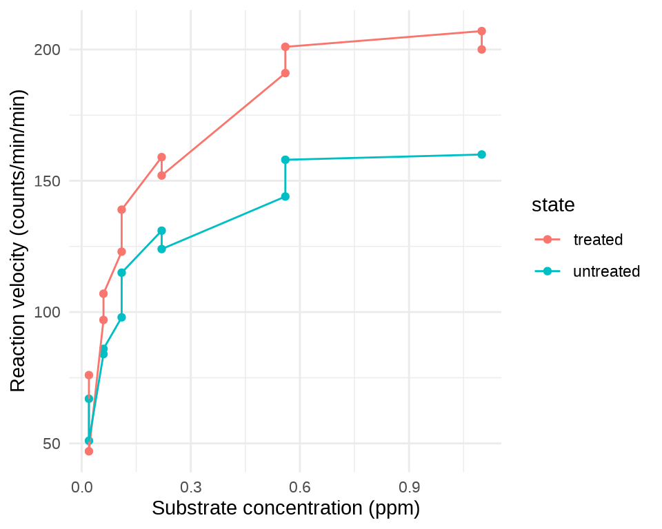
基于数据集 Puromycin 分析酶促反应的反应速率(提示:Michaelis-Menten 模型和函数
SSmicmen())。 -
基于 MASS 包的地形数据集 topo,建立高斯过程回归模型,比较贝叶斯预测与克里金插值预测的效果。
代码
data(topo, package = "MASS")
set.seed(20232023)
nchains <- 2 # 2 条迭代链
# 给每条链设置不同的参数初始值
inits_data_gaussian <- lapply(1:nchains, function(i) {
  list(
    beta = rnorm(1),
    sigma = runif(1),
    phi = runif(1),
    tau = runif(1)
  )
})
# 预测区域网格化
nx <- ny <- 27
topo_grid_df <- expand.grid(
  x = seq(from = 0, to = 6.5, length.out = nx),
  y = seq(from = 0, to = 6.5, length.out = ny)
)
# 对数高斯模型
topo_gaussian_d <- list(
  N1 = nrow(topo), # 观测记录的条数
  N2 = nrow(topo_grid_df),
  D = 2, # 2 维坐标
  x1 = topo[, c("x", "y")], # N x 2 坐标矩阵
  x2 = topo_grid_df[, c("x", "y")],
  y1 = topo[, "z"] # N 向量
)
library(cmdstanr)
# 编码
mod_topo_gaussian <- cmdstan_model(
  stan_file = "code/gaussian_process_pred.stan",
  compile = TRUE, cpp_options = list(stan_threads = TRUE)
)
# 高斯过程回归模型
fit_topo_gaussian <- mod_topo_gaussian$sample(
  data = topo_gaussian_d,   # 观测数据
  init = inits_data_gaussian,   # 迭代初值
  iter_warmup = 500,            # 每条链预处理迭代次数
  iter_sampling = 1000,         # 每条链总迭代次数
  chains = nchains,             # 马尔科夫链的数目
  parallel_chains = 2,      # 指定 CPU 核心数,可以给每条链分配一个
  threads_per_chain = 1,    # 每条链设置一个线程
  show_messages = FALSE,    # 不显示迭代的中间过程
  refresh = 0,              # 不显示采样的进度
  output_dir = "data-raw/",
  seed = 20232023
)
# 诊断
fit_topo_gaussian$diagnostic_summary()
# 对数高斯模型
fit_topo_gaussian$summary(
  variables = c("lp__", "beta", "sigma", "phi", "tau"),
  .num_args = list(sigfig = 4, notation = "dec")
)
# 未采样的位置的预测值
ypred <- fit_topo_gaussian$summary(variables = "ypred", "mean")
# 预测值
topo_grid_df$ypred <- ypred$mean
# 整理数据
library(sf)
topo_grid_sf <- st_as_sf(topo_grid_df, coords = c("x", "y"), dim = "XY")
library(stars)
# 26x26 的网格
topo_grid_stars <- st_rasterize(topo_grid_sf, nx = 26, ny = 26)

library(ggplot2)
ggplot() +
  geom_stars(data = topo_grid_stars, aes(fill = ypred)) +
  scale_fill_viridis_c(option = "C") +
  theme_bw()