39  时间序列回归

library(cmdstanr)
library(zoo)
library(xts) # xts 依赖 zoo
library(fGarch)
library(INLA)
library(mgcv)
library(tensorflow)
library(ggplot2)
library(bayesplot)

39.1 随机波动率模型

随机波动率模型主要用于股票时间序列数据建模。本节以美团股价数据为例介绍随机波动率模型，并分别以 Stan 框架和 fGarch 包拟合模型。

# 美团上市至 2023-07-15
meituan <- readRDS(file = "data/meituan.rds")
library(zoo)
library(xts)
library(ggplot2)
autoplot(meituan[, "3690.HK.Adjusted"]) +
  theme_classic() +
  labs(x = "日期", y = "股价")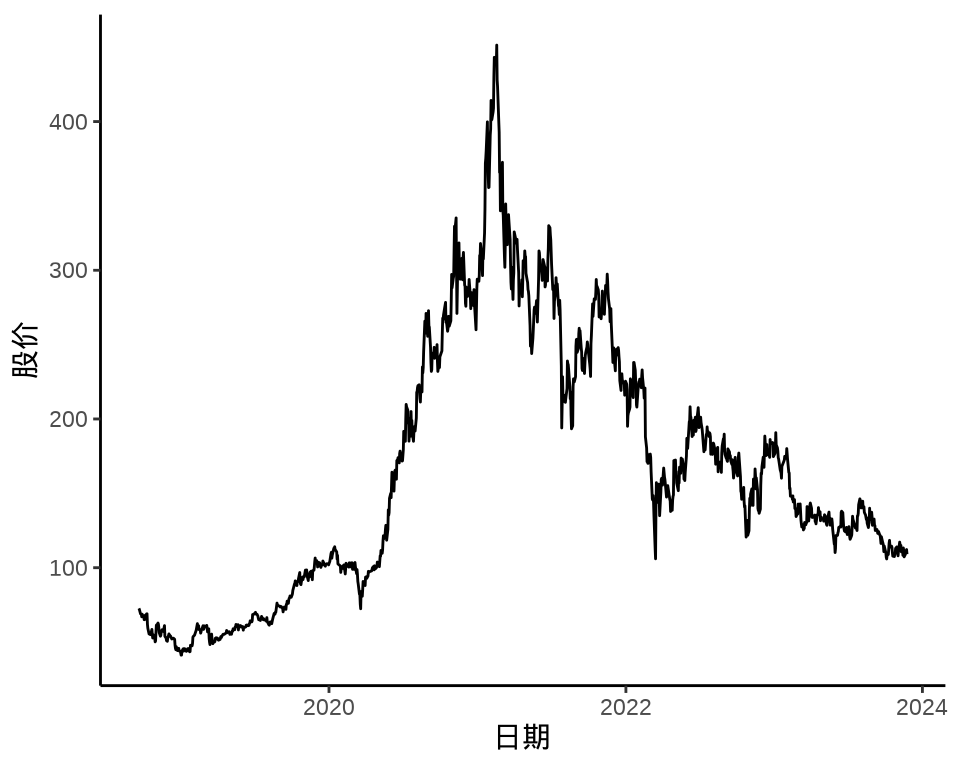

图 39.1: 美团股价走势

对数收益率的计算公式如下：

\[ \mathrm{对数收益率} = \ln(\mathrm{今日收盘价} / \mathrm{上一收盘价} ) = \ln (1 + \mathrm{普通收益率}) \]

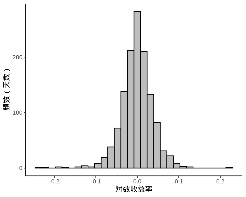
下图给出股价对数收益率变化和股价对数收益率的分布，可以看出在不同时间段，收益率波动幅度是不同的，美团股价对数收益率的分布可以看作正态分布。

meituan_log_return <- log(1 + diff(meituan[, "3690.HK.Adjusted"]) /  meituan[, "3690.HK.Adjusted"])[-1,]
autoplot(meituan_log_return) +
  theme_classic() +
  labs(x = "日期", y = "对数收益率")
ggplot(data = meituan_log_return, aes(x = `3690.HK.Adjusted`)) +
  geom_histogram(color = "black", fill = "gray", bins = 30) +
  theme_classic() +
  labs(x = "对数收益率", y = "频数（天数）")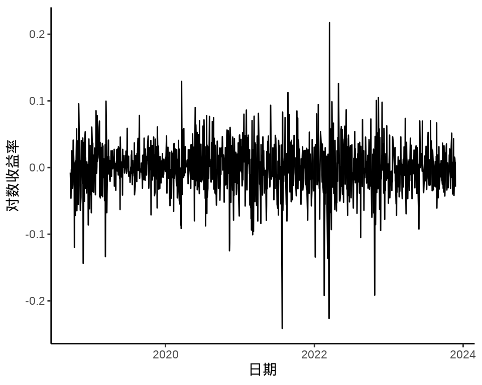

(a) 对数收益率的变动

(b) 对数收益率的分布

图 39.2: 美团股价对数收益率的情况

检查对数收益率序列的自相关图

acf(meituan_log_return, main = "")

图 39.3: 对数收益率的自相关图

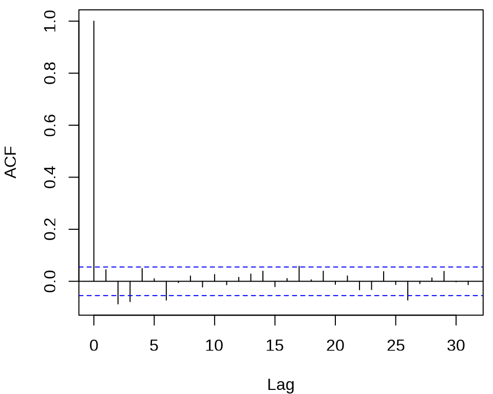
发现，滞后 2、3、6、26 阶都有出界，滞后 17 阶略微出界，其它的自相关都在零水平线的界限内。

Box.test(meituan_log_return, lag = 12, type = "Ljung")

#> 
#>  Box-Ljung test
#> 
#> data:  meituan_log_return
#> X-squared = 32.367, df = 12, p-value = 0.001214

在 0.05 水平下拒绝了白噪声检验，说明对数收益率序列存在相关性。同理，也注意到对数收益率的绝对值和平方序列都不是独立的，存在相关性。

# ARCH 效应的检验
Box.test((meituan_log_return - mean(meituan_log_return))^2, lag = 12, type = "Ljung")

#> 
#>  Box-Ljung test
#> 
#> data:  (meituan_log_return - mean(meituan_log_return))^2
#> X-squared = 113.76, df = 12, p-value < 2.2e-16

结果高度显著，说明有 ARCH 效应。

39.1.1 Stan 框架

library(cmdstanr)

39.1.2 fGarch 包

《金融时间序列分析讲义》两个波动率建模方法

• 自回归条件异方差模型（Autoregressive Conditional Heteroskedasticity，简称 ARCH）。
• 广义自回归条件异方差模型 （Generalized Autoregressive Conditional Heteroskedasticity，简称 GARCH ）

确定 ARCH 模型的阶，观察残差的平方的 ACF 和 PACF 。

acf((meituan_log_return - mean(meituan_log_return))^2, main = "")
pacf((meituan_log_return - mean(meituan_log_return))^2, main = "")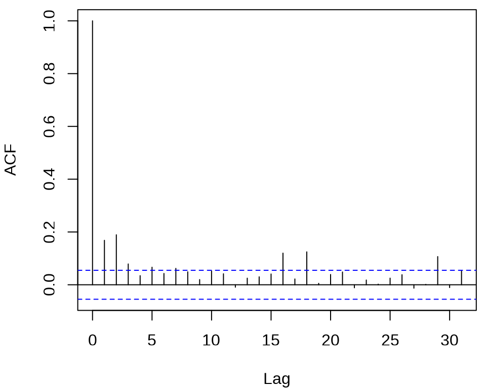

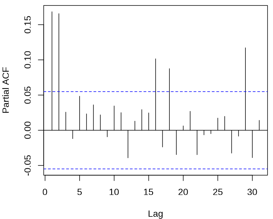
(a) 自相关图

(b) 偏自相关图

图 39.4: 对数收益率的残差平方

发现 ACF 在滞后 1、2、3 阶比较突出，PACF 在滞后 1、2、16、18、29 阶比较突出。所以下面先来考虑低阶的 ARCH(2) 模型，设 \(r_t\) 为对数收益率。

\[ \begin{aligned} r_t &= \mu + a_t, \quad a_t = \sigma_t \epsilon_t, \quad \epsilon_t \sim \mathcal{N}(0,1) \\ \sigma_t^2 &= \alpha_0 + \alpha_1 a_{t-1}^2 + \alpha_2 a_{t-2}^2. \end{aligned} \]

拟合 ARCH 模型，比较模型估计结果，根据系数显著性的结果，采纳 ARCH(2) 模型。

library(fGarch)
meituan_garch1 <- garchFit(~ 1 + garch(2, 0), data = meituan_log_return, trace = FALSE, cond.dist = "std")
summary(meituan_garch1)

#> 
#> Title:
#>  GARCH Modelling 
#> 
#> Call:
#>  garchFit(formula = ~1 + garch(2, 0), data = meituan_log_return, 
#>     cond.dist = "std", trace = FALSE) 
#> 
#> Mean and Variance Equation:
#>  data ~ 1 + garch(2, 0)
#> <environment: 0x5579d2fa0248>
#>  [data = meituan_log_return]
#> 
#> Conditional Distribution:
#>  std 
#> 
#> Coefficient(s):
#>          mu        omega       alpha1       alpha2        shape  
#> -5.6632e-05   1.0704e-03   1.1555e-01   1.4380e-01   4.8131e+00  
#> 
#> Std. Errors:
#>  based on Hessian 
#> 
#> Error Analysis:
#>          Estimate  Std. Error  t value Pr(>|t|)    
#> mu     -5.663e-05   8.881e-04   -0.064  0.94915    
#> omega   1.070e-03   9.507e-05   11.260  < 2e-16 ***
#> alpha1  1.156e-01   4.299e-02    2.688  0.00719 ** 
#> alpha2  1.438e-01   4.754e-02    3.025  0.00249 ** 
#> shape   4.813e+00   6.561e-01    7.336  2.2e-13 ***
#> ---
#> Signif. codes:  0 '***' 0.001 '**' 0.01 '*' 0.05 '.' 0.1 ' ' 1
#> 
#> Log Likelihood:
#>  2459.91    normalized:  1.930856 
#> 
#> Description:
#>  Sun Dec 10 15:29:12 2023 by user:  
#> 
#> 
#> Standardised Residuals Tests:
#>                                   Statistic      p-Value
#>  Jarque-Bera Test   R    Chi^2  632.2496448 0.000000e+00
#>  Shapiro-Wilk Test  R    W        0.9648585 0.000000e+00
#>  Ljung-Box Test     R    Q(10)   19.3876684 3.560618e-02
#>  Ljung-Box Test     R    Q(15)   23.5920804 7.235243e-02
#>  Ljung-Box Test     R    Q(20)   33.2714312 3.149690e-02
#>  Ljung-Box Test     R^2  Q(10)   12.6594516 2.433403e-01
#>  Ljung-Box Test     R^2  Q(15)   25.3895008 4.495082e-02
#>  Ljung-Box Test     R^2  Q(20)   57.7893864 1.556847e-05
#>  LM Arch Test       R    TR^2    17.7056006 1.249263e-01
#> 
#> Information Criterion Statistics:
#>       AIC       BIC       SIC      HQIC 
#> -3.853862 -3.833650 -3.853893 -3.846271

函数 garchFit() 的参数 cond.dist 默认值为 "norm" 表示标准正态分布，cond.dist = "std" 表示标准 t 分布。模型均值的估计值接近 0 是符合预期的，且显著性没通过，对数收益率在 0 上下波动。将估计结果代入模型，得到

\[ \begin{aligned} r_t &= -5.665 \times 10^{-5} + a_t, \quad a_t = \sigma_t \epsilon_t, \quad \epsilon_t \sim \mathcal{N}(0,1) \\ \sigma_t^2 &= 1.070 \times 10^{-3} + 0.1156 a_{t-1}^2 + 0.1438a_{t-2}^2. \end{aligned} \]

下面考虑 GARCH(1,1) 模型

\[ \begin{aligned} r_t &= \mu + a_t, \quad a_t = \sigma_t \epsilon_t, \quad \epsilon_t \sim \mathcal{N}(0,1) \\ \sigma_t^2 &= \alpha_0 + \alpha_1 a_{t-1}^2 + \beta_1 \sigma_{t-1}^2. \end{aligned} \]

meituan_garch2 <- garchFit(~ 1 + garch(1, 1), data = meituan_log_return, trace = FALSE, cond.dist = "std")
summary(meituan_garch2)

#> 
#> Title:
#>  GARCH Modelling 
#> 
#> Call:
#>  garchFit(formula = ~1 + garch(1, 1), data = meituan_log_return, 
#>     cond.dist = "std", trace = FALSE) 
#> 
#> Mean and Variance Equation:
#>  data ~ 1 + garch(1, 1)
#> <environment: 0x5579d0431d08>
#>  [data = meituan_log_return]
#> 
#> Conditional Distribution:
#>  std 
#> 
#> Coefficient(s):
#>          mu        omega       alpha1        beta1        shape  
#> -8.6653e-05   3.4394e-05   5.8249e-02   9.1819e-01   5.2787e+00  
#> 
#> Std. Errors:
#>  based on Hessian 
#> 
#> Error Analysis:
#>          Estimate  Std. Error  t value Pr(>|t|)    
#> mu     -8.665e-05   8.641e-04   -0.100  0.92012    
#> omega   3.439e-05   1.866e-05    1.843  0.06529 .  
#> alpha1  5.825e-02   1.788e-02    3.257  0.00113 ** 
#> beta1   9.182e-01   2.667e-02   34.434  < 2e-16 ***
#> shape   5.279e+00   7.517e-01    7.023 2.18e-12 ***
#> ---
#> Signif. codes:  0 '***' 0.001 '**' 0.01 '*' 0.05 '.' 0.1 ' ' 1
#> 
#> Log Likelihood:
#>  2478.786    normalized:  1.945672 
#> 
#> Description:
#>  Sun Dec 10 15:29:12 2023 by user:  
#> 
#> 
#> Standardised Residuals Tests:
#>                                   Statistic   p-Value
#>  Jarque-Bera Test   R    Chi^2  523.6362720 0.0000000
#>  Shapiro-Wilk Test  R    W        0.9666878 0.0000000
#>  Ljung-Box Test     R    Q(10)   14.4633761 0.1528851
#>  Ljung-Box Test     R    Q(15)   18.5039288 0.2370994
#>  Ljung-Box Test     R    Q(20)   27.4217443 0.1238100
#>  Ljung-Box Test     R^2  Q(10)    8.7555217 0.5554521
#>  Ljung-Box Test     R^2  Q(15)   10.6532128 0.7767678
#>  Ljung-Box Test     R^2  Q(20)   23.7435667 0.2537732
#>  LM Arch Test       R    TR^2    10.1204846 0.6053914
#> 
#> Information Criterion Statistics:
#>       AIC       BIC       SIC      HQIC 
#> -3.883494 -3.863283 -3.883525 -3.875903

波动率的贡献主要来自 \(\sigma_{t-1}^2\) ，其系数 \(\beta_1\) 为 0.918。通过对数似然的比较，可以发现 GARCH(1,1) 模型比 ARCH(2) 模型更好。

39.2 贝叶斯可加模型

大规模时间序列回归，观察值是比较多的，可达数十万、数百万，乃至更多。粗粒度时时间跨度往往很长，比如数十年的天粒度数据，细粒度时时间跨度可短可长，比如数年的半小时级数据，总之，需要包含多个季节的数据，各种季节性重复出现。通过时序图可以观察到明显的季节性，而且往往是多种周期不同的季节性混合在一起，有时还包含一定的趋势性。举例来说，比如 2018-2023 年美国旧金山犯罪事件报告数据，事件数量的变化趋势，除了上述季节性因素，特殊事件疫情肯定会影响，数据规模约 200 M 。再比如 2018-2023 年美国境内和跨境旅游业中的航班数据，原始数据非常大，R 包 nycflights13 提供纽约机场的部分航班数据。

39.2.1 Stan 框架

library(cmdstanr)

39.2.2 INLA 框架

模型内容、成分结构和参数解释

阿卜杜拉国王科技大学（King Abdullah University of Science and Technology 简称 KAUST）的 Håvard Rue 等开发了 INLA 框架 (Rue, Martino, 和 Chopin 2009)。INLA 动态时间序列建模 (Nalini Ravishanker 和 Soyer 2022)

library(INLA)

39.3 一些非参数模型

39.3.1 mgcv 包

模型内容、成分结构和参数解释。一般可加模型，在似然函数中添加平滑样条，与 Lasso 回归模型在形式上有相似之处，属于频率派方法。

mgcv 包 (S. N. Wood 2017) 是 R 软件内置的推荐组件，由 Simon Wood 开发和维护，历经多年，成熟稳定。对于时间序列数据预测，数万和百万级观测值都可以 (Simon N. Wood, Goude, 和 Shaw 2015)。函数 bam()

library(mgcv)

39.3.2 nnet 包

多层感知机是一种前馈神经网络，nnet 包的函数 nnet() 实现了单隐藏层的简单神经网络。

# library(nnet) 

39.3.3 tensorflow 框架

前面介绍的模型都具有非常强的可解释性，比如各个参数对模型的作用。对于复杂的时间序列数据，比较适合用复杂的模型来拟合，看重模型的泛化能力，而不那么关注模型的机理。下面用 LSTM （长短期记忆）神经网络来训练时间序列数据，预测未来一周的趋势。

library(tensorflow)
# tf$abs(x = c(-1, 1, 2))

forecastML 采用机器学习方法可以一次向前预测多期。

39.4 习题

1. 基于 R 软件内置的数据集 sunspots 和 sunspot.month 比较 INLA 和 mgcv 框架的预测效果。

   sunspots_tbl <- broom::tidy(sunspots)
   sunspots_month_tbl <- broom::tidy(sunspot.month)
   ggplot() +
     geom_line(data = sunspots_month_tbl, aes(x = index, y = value), color = "red") +
     geom_line(data = sunspots_tbl, aes(x = index, y = value)) +
     theme_bw() +
     labs(x = "年月", y = "数量")

   

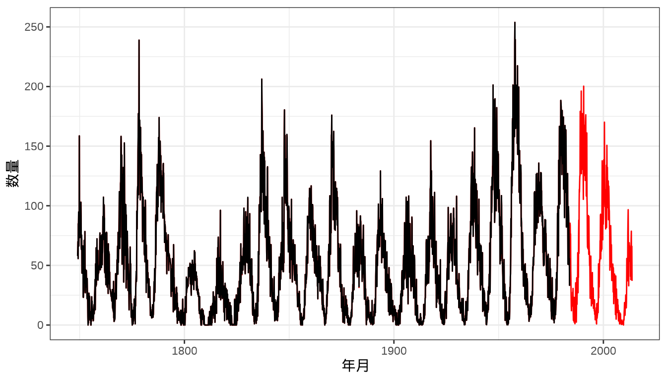
   图 39.5: 预测月粒度太阳黑子数量

   图中黑线和红线分别表示 1749-1983 年、1984-2014 年每月太阳黑子数量。

Nalini Ravishanker, Balaji Raman, 和 Refik Soyer. 2022. Dynamic Time Series Models using R-INLA: An Applied Perspective. Boca Raton, Florida: Chapman; Hall/CRC. https://ramanbala.github.io/dynamic-time-series-models-R-INLA/.

Rue, Håvard, Sara Martino, 和 Nicholas Chopin. 2009. 《Approximate Bayesian Inference for Latent Gaussian Models Using Integrated Nested Laplace Approximations (with discussion)》. Journal of the Royal Statistical Society, Series B 71 (2): 319–92.

Wood, S. N. 2017. Generalized Additive Models: An Introduction with R. 2nd 本. Chapman; Hall/CRC. https://www.maths.ed.ac.uk/~swood34/igam/.

Wood, Simon N., Yannig Goude, 和 Simon Shaw. 2015. 《Generalized Additive Models for Large Data Sets》. Journal of the Royal Statistical Society Series C: Applied Statistics 64 (1): 139–55. https://doi.org/10.1111/rssc.12068.