37 广义可加模型
相比于广义线性模型,广义可加模型可以看作是一种非线性模型,模型中含有非线性的成分。
- 多元适应性(自适应)回归样条 multivariate adaptive regression splines
- Friedman, Jerome H. 1991. Multivariate Adaptive Regression Splines. The Annals of Statistics. 19(1):1–67. https://doi.org/10.1214/aos/1176347963
- earth: Multivariate Adaptive Regression Splines http://www.milbo.users.sonic.net/earth
- Friedman, Jerome H. 2001. Greedy function approximation: A gradient boosting machine. The Annals of Statistics. 29(5):1189–1232. https://doi.org/10.1214/aos/1013203451
- Friedman, Jerome H., Trevor Hastie and Robert Tibshirani. Additive Logistic Regression: A Statistical View of Boosting. The Annals of Statistics. 28(2): 337–374. http://www.jstor.org/stable/2674028
- Flexible Modeling of Alzheimer’s Disease Progression with I-Splines PDF 文档
- Implementation of B-Splines in Stan 网页文档
37.1 案例:模拟摩托车事故
37.1.1 mgcv
MASS 包的 mcycle 数据集
#> 'data.frame':    133 obs. of  2 variables:
#>  $ times: num  2.4 2.6 3.2 3.6 4 6.2 6.6 6.8 7.8 8.2 ...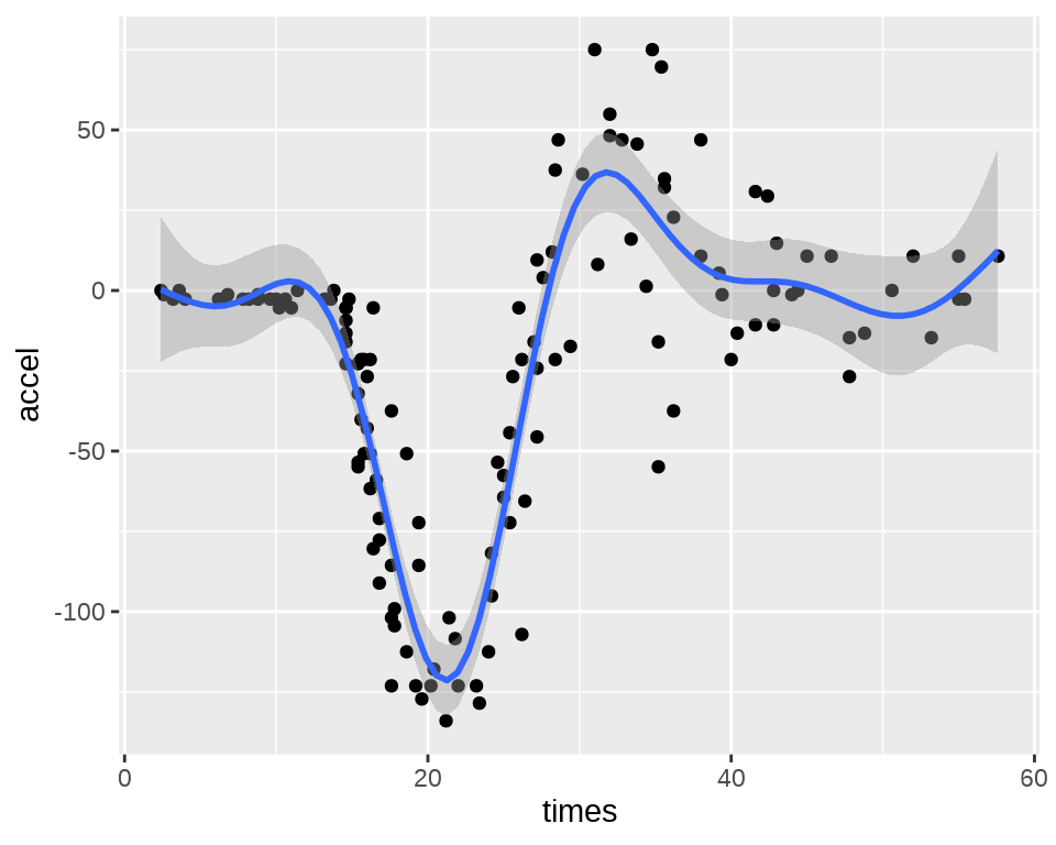
#> $ accel: num 0 -1.3 -2.7 0 -2.7 -2.7 -2.7 -1.3 -2.7 -2.7 ...library(ggplot2)
ggplot(data = mcycle, aes(x = times, y = accel)) +
geom_point() +
theme_classic() +
labs(x = "时间(ms)", y = "加速度(g)")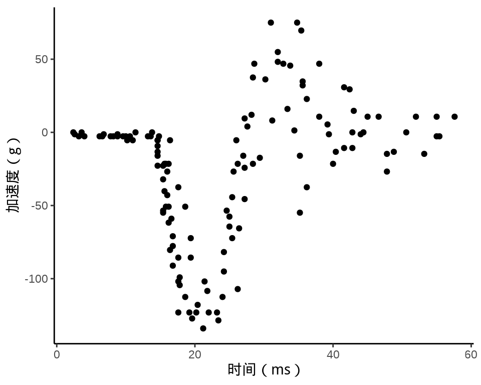
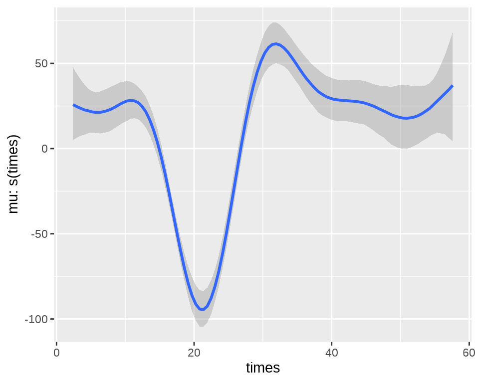
样条回归
library(mgcv)
mcycle_mgcv <- gam(accel ~ s(times), data = mcycle, method = "REML")
summary(mcycle_mgcv)
#>
#> Family: gaussian
#> Link function: identity
#>
#> Formula:
#> accel ~ s(times)
#>
#> Parametric coefficients:
#> Estimate Std. Error t value Pr(>|t|)
#> (Intercept) -25.546 1.951 -13.09 <2e-16 ***
#> ---
#> Signif. codes: 0 '***' 0.001 '**' 0.01 '*' 0.05 '.' 0.1 ' ' 1
#>
#> Approximate significance of smooth terms:
#> edf Ref.df F p-value
#> s(times) 8.625 8.958 53.4 <2e-16 ***
#> ---
#> Signif. codes: 0 '***' 0.001 '**' 0.01 '*' 0.05 '.' 0.1 ' ' 1
#>
#> R-sq.(adj) = 0.783 Deviance explained = 79.7%
#> -REML = 616.14 Scale est. = 506.35 n = 133方差成分
#>
#> Standard deviations and 0.95 confidence intervals:
#>
#>            std.dev     lower      upper
#> s(times) 807.88726 480.66162 1357.88215
#> scale     22.50229  19.85734   25.49954
#>
#> Rank: 2/2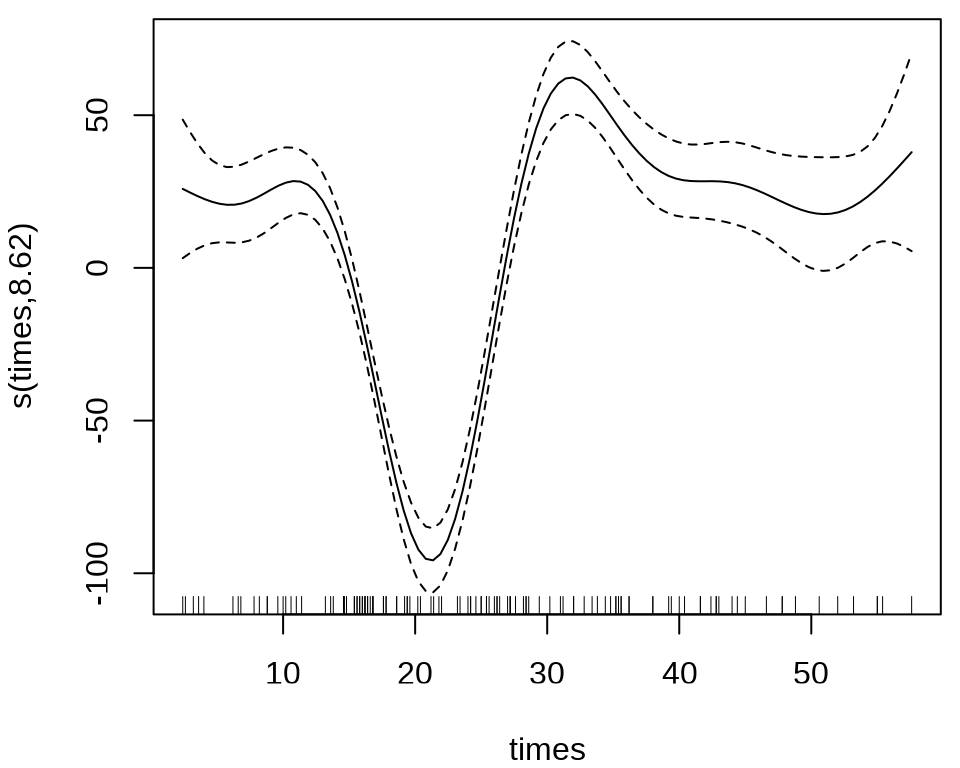
ggplot2 包的平滑图层函数 geom_smooth() 集成了 mgcv 包的函数 gam() 的功能。
37.1.2 cmdstanr
37.1.3 rstanarm
rstanarm 可以拟合一般的广义可加(混合)模型。
Model Info:
 function:     stan_gamm4
 family:       gaussian [identity]
 formula:      accel ~ s(times)
 algorithm:    sampling
 sample:       1200 (posterior sample size)
 priors:       see help('prior_summary')
 observations: 133

Estimates:
                       mean    sd      10%     50%     90%
(Intercept)            -25.6     2.1   -28.4   -25.5   -23.0
s(times).1             340.4   232.9    61.1   340.8   634.7
s(times).2           -1218.9   243.3 -1529.2 -1218.8  -913.5
s(times).3            -567.8   147.0  -765.2  -567.1  -385.3
s(times).4            -619.8   133.8  -791.1  -617.0  -458.9
s(times).5           -1056.2    85.8 -1162.8 -1055.7  -945.1
s(times).6             -89.2    49.8  -154.4   -89.4   -27.6
s(times).7            -232.2    33.8  -274.7  -232.2  -189.5
s(times).8              17.3   105.8  -121.0    15.5   150.1
s(times).9               4.1    33.1   -25.8     1.0    39.1
sigma                   24.7     1.6    22.6    24.6    26.8
smooth_sd[s(times)1]   399.9    59.2   327.6   395.4   479.1
smooth_sd[s(times)2]    25.2    25.4     2.9    17.5    56.6

Fit Diagnostics:
           mean   sd    10%   50%   90%
mean_PPD -25.5    3.0 -29.3 -25.5 -21.8

The mean_ppd is the sample average posterior predictive distribution of the outcome variable (for details see help('summary.stanreg')).

MCMC diagnostics
                     mcse Rhat n_eff
(Intercept)          0.1  1.0  1052
s(times).1           7.0  1.0  1103
s(times).2           6.7  1.0  1329
s(times).3           4.4  1.0  1101
s(times).4           3.8  1.0  1230
s(times).5           2.5  1.0  1137
s(times).6           1.5  1.0  1128
s(times).7           1.0  1.0  1062
s(times).8           3.1  1.0  1147
s(times).9           1.0  1.0  1052
sigma                0.0  1.0  1154
smooth_sd[s(times)1] 1.8  1.0  1136
smooth_sd[s(times)2] 0.7  1.0  1157
mean_PPD             0.1  1.0   997
log-posterior        0.1  1.0  1122

For each parameter, mcse is Monte Carlo standard error, n_eff is a crude measure of effective sample size, and Rhat is the potential scale reduction factor on split chains (at convergence Rhat=1).
计算 LOO 值
Computed from 1200 by 133 log-likelihood matrix

         Estimate   SE
elpd_loo   -611.0  8.8
p_loo         7.3  1.2
looic      1222.0 17.5
------
Monte Carlo SE of elpd_loo is 0.1.

All Pareto k estimates are good (k < 0.5).
See help('pareto-k-diagnostic') for details.37.1.4 brms
另一个综合型的贝叶斯分析扩展包是 brms 包
# 拟合模型
mcycle_brms <- brms::brm(accel ~ s(times),
  data = mcycle, family = gaussian(), cores = 2, seed = 20232023,
  iter = 4000, warmup = 1000, thin = 10, refresh = 0, silent = 2,
  control = list(adapt_delta = 0.99)
)
# 模型输出
summary(mcycle_brms)
#> Family: gaussian
#> Links: mu = identity; sigma = identity
#> Formula: accel ~ s(times)
#> Data: mcycle (Number of observations: 133)
#> Draws: 4 chains, each with iter = 4000; warmup = 1000; thin = 10;
#> total post-warmup draws = 1200
#>
#> Smooth Terms:
#> Estimate Est.Error l-95% CI u-95% CI Rhat Bulk_ESS Tail_ESS
#> sds(stimes_1) 721.87 180.77 458.68 1121.47 1.00 1286 1201
#>
#> Population-Level Effects:
#> Estimate Est.Error l-95% CI u-95% CI Rhat Bulk_ESS Tail_ESS
#> Intercept -25.41 1.94 -29.23 -21.43 1.00 1063 1049
#> stimes_1 123.64 291.52 -443.35 720.84 1.00 1127 1170
#>
#> Family Specific Parameters:
#> Estimate Est.Error l-95% CI u-95% CI Rhat Bulk_ESS Tail_ESS
#> sigma 22.70 1.45 19.90 25.71 1.00 1183 1260
#>
#> Draws were sampled using sampling(NUTS). For each parameter, Bulk_ESS
#> and Tail_ESS are effective sample size measures, and Rhat is the potential
#> scale reduction factor on split chains (at convergence, Rhat = 1).固定效应
#>           Estimate  Est.Error       Q2.5     Q97.5
#> Intercept -25.4117   1.938916  -29.22722 -21.43478
#> stimes_1  123.6444 291.516658 -443.34899 720.83720
LOO 值与 rstanarm 包计算的值很接近。
#>
#> Computed from 1200 by 133 log-likelihood matrix
#>
#>          Estimate   SE
#> elpd_loo   -608.5 10.3
#> p_loo         9.1  1.6
#> looic      1216.9 20.6
#> ------
#> Monte Carlo SE of elpd_loo is 0.1.
#>
#> Pareto k diagnostic values:
#>                          Count Pct.    Min. n_eff
#> (-Inf, 0.5]   (good)     132   99.2%   317
#>  (0.5, 0.7]   (ok)         1    0.8%   795
#>    (0.7, 1]   (bad)        0    0.0%   <NA>
#>    (1, Inf)   (very bad)   0    0.0%   <NA>
#>
#> All Pareto k estimates are ok (k < 0.7).
#> See help('pareto-k-diagnostic') for details.
模型中样条平滑的效应
37.1.5 GINLA
mgcv 包的简化版 INLA 算法用于贝叶斯计算
library(mgcv)
mcycle_mgcv <- gam(accel ~ s(times), data = mcycle, fit = FALSE)
# 简化版 INLA
mcycle_ginla <- ginla(G = mcycle_mgcv)
str(mcycle_ginla)
#> List of 2
#> $ density: num [1:10, 1:100] 2.04e-04 2.13e-05 8.21e-06 3.47e-05 1.14e-05 ...
#> $ beta : num [1:10, 1:100] -32.8 -133.4 -139.4 -152.5 -153.3 ...提取最大后验估计
37.1.6 INLA
37.2 案例:朗格拉普岛核污染
从线性到可加,意味着从线性到非线性,可加模型容纳非线性的成分,比如高斯过程、样条。
37.2.1 mgcv
本节复用 章节 28 朗格拉普岛核污染数据,相关背景不再赘述,下面首先加载数据到 R 环境。
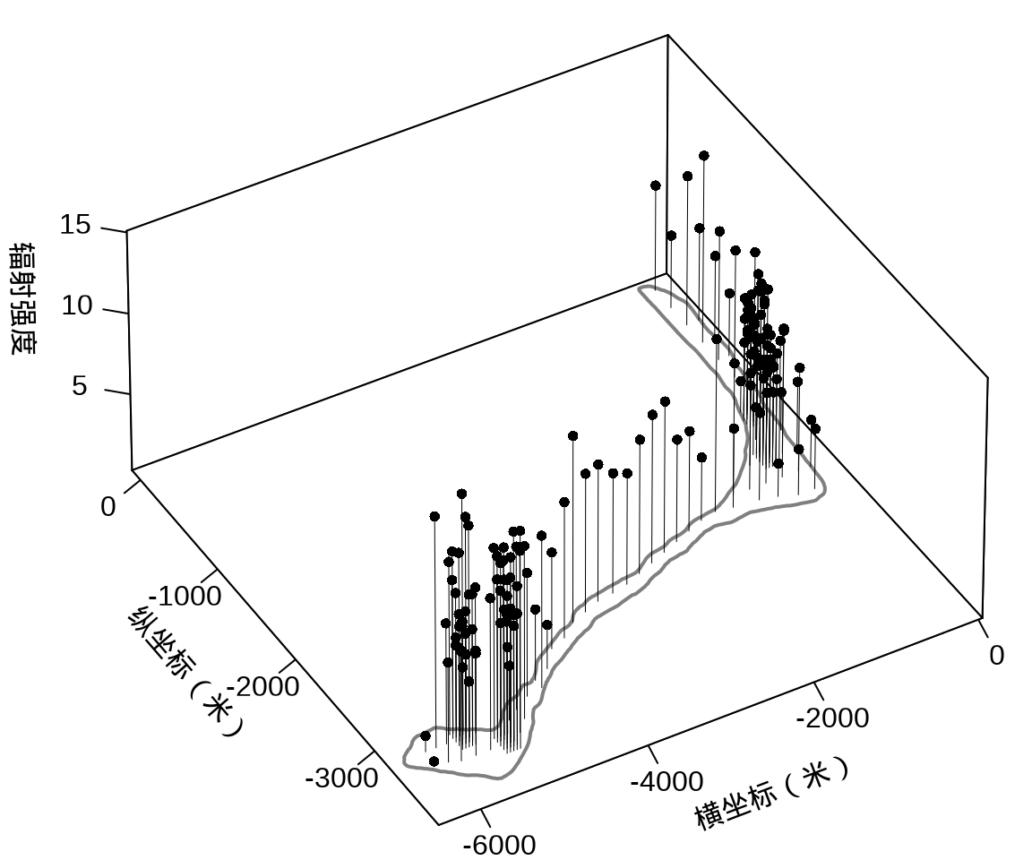
接着,将岛上各采样点的辐射强度展示出来,算是简单回顾一下数据概况。
代码
library(plot3D)
with(rongelap, {
  opar <- par(mar = c(.1, 2.5, .1, .1), no.readonly = TRUE)
  rongelap_coastline$cZ <- 0
  scatter3D(
    x = cX, y = cY, z = counts / time,
    xlim = c(-6500, 50), ylim = c(-3800, 110),
    xlab = "\n横坐标(米)", ylab = "\n纵坐标(米)",
    zlab = "\n辐射强度", lwd = 0.5, cex = 0.8,
    pch = 16, type = "h", ticktype = "detailed",
    phi = 40, theta = -30, r = 50, d = 1,
    expand = 0.5, box = TRUE, bty = "b",
    colkey = F, col = "black",
    panel.first = function(trans) {
      XY <- trans3D(
        x = rongelap_coastline$cX,
        y = rongelap_coastline$cY,
        z = rongelap_coastline$cZ,
        pmat = trans
      )
      lines(XY, col = "gray50", lwd = 2)
    }
  )
  rongelap_coastline$cZ <- NULL
  on.exit(par(opar), add = TRUE)
})
在这里,从广义可加混合效应模型的角度来对核污染数据建模,空间效应仍然是用高斯过程来表示,响应变量服从带漂移项的泊松分布。采用 mgcv 包 (S. N. Wood 2004) 的函数 gam() 拟合模型,其中,含 49 个参数的样条近似高斯过程,高斯过程的核函数为默认的梅隆型。更多详情见 mgcv 包的函数 s() 帮助文档参数的说明,默认值是梅隆型相关函数及默认的范围参数,作者自己定义了一套符号约定。
library(nlme)
library(mgcv)
fit_rongelap_gam <- gam(
  counts ~ s(cX, cY, bs = "gp", k = 50), offset = log(time),
  data = rongelap, family = poisson(link = "log")
)
# 模型输出
summary(fit_rongelap_gam)
#>
#> Family: poisson
#> Link function: log
#>
#> Formula:
#> counts ~ s(cX, cY, bs = "gp", k = 50)
#>
#> Parametric coefficients:
#> Estimate Std. Error z value Pr(>|z|)
#> (Intercept) 1.976815 0.001642 1204 <2e-16 ***
#> ---
#> Signif. codes: 0 '***' 0.001 '**' 0.01 '*' 0.05 '.' 0.1 ' ' 1
#>
#> Approximate significance of smooth terms:
#> edf Ref.df Chi.sq p-value
#> s(cX,cY) 48.98 49 34030 <2e-16 ***
#> ---
#> Signif. codes: 0 '***' 0.001 '**' 0.01 '*' 0.05 '.' 0.1 ' ' 1
#>
#> R-sq.(adj) = 0.876 Deviance explained = 60.7%
#> UBRE = 153.78 Scale est. = 1 n = 157#> s(cX,cY)
#> 2543.376值得一提的是核函数的类型和默认参数的选择,参数 m 接受一个向量, m[1] 取值为 1 至 5,分别代表球型 spherical, 幂指数 power exponential 和梅隆型 Matern with \(\kappa\) = 1.5, 2.5 or 3.5 等 5 种相关/核函数。
接下来,基于岛屿的海岸线数据划分出网格,将格点作为新的预测位置。
#> Linking to GEOS 3.10.1, GDAL 3.4.3, PROJ 8.2.0; sf_use_s2() is TRUElibrary(abind)
library(stars)
# 类型转化
rongelap_sf <- st_as_sf(rongelap, coords = c("cX", "cY"), dim = "XY")
rongelap_coastline_sf <- st_as_sf(rongelap_coastline, coords = c("cX", "cY"), dim = "XY")
rongelap_coastline_sfp <- st_cast(st_combine(st_geometry(rongelap_coastline_sf)), "POLYGON")
# 添加缓冲区
rongelap_coastline_buffer <- st_buffer(rongelap_coastline_sfp, dist = 50)
# 构造带边界约束的网格
rongelap_coastline_grid <- st_make_grid(rongelap_coastline_buffer, n = c(150, 75))
# 将 sfc 类型转化为 sf 类型
rongelap_coastline_grid <- st_as_sf(rongelap_coastline_grid)
rongelap_coastline_buffer <- st_as_sf(rongelap_coastline_buffer)
rongelap_grid <- rongelap_coastline_grid[rongelap_coastline_buffer, op = st_intersects]
# 计算网格中心点坐标
rongelap_grid_centroid <- st_centroid(rongelap_grid)
# 共计 1612 个预测点
rongelap_grid_df <- as.data.frame(st_coordinates(rongelap_grid_centroid))
colnames(rongelap_grid_df) <- c("cX", "cY")模型对象 fit_rongelap_gam 在新的格点上预测核辐射强度,接着整理预测结果数据。
# 预测
rongelap_grid_df$ypred <- as.vector(predict(fit_rongelap_gam, newdata = rongelap_grid_df, type = "response"))
# 整理预测数据
rongelap_grid_sf <- st_as_sf(rongelap_grid_df, coords = c("cX", "cY"), dim = "XY")
rongelap_grid_stars <- st_rasterize(rongelap_grid_sf, nx = 150, ny = 75)
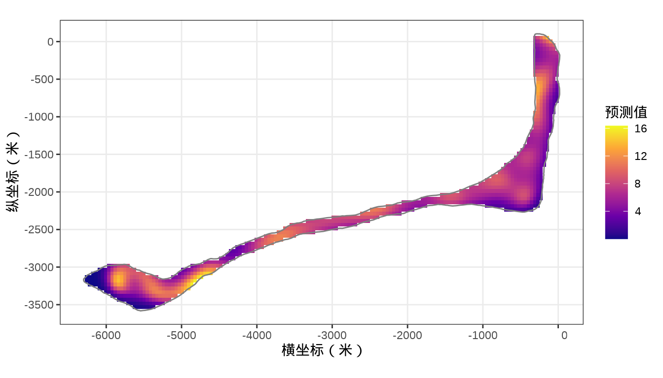
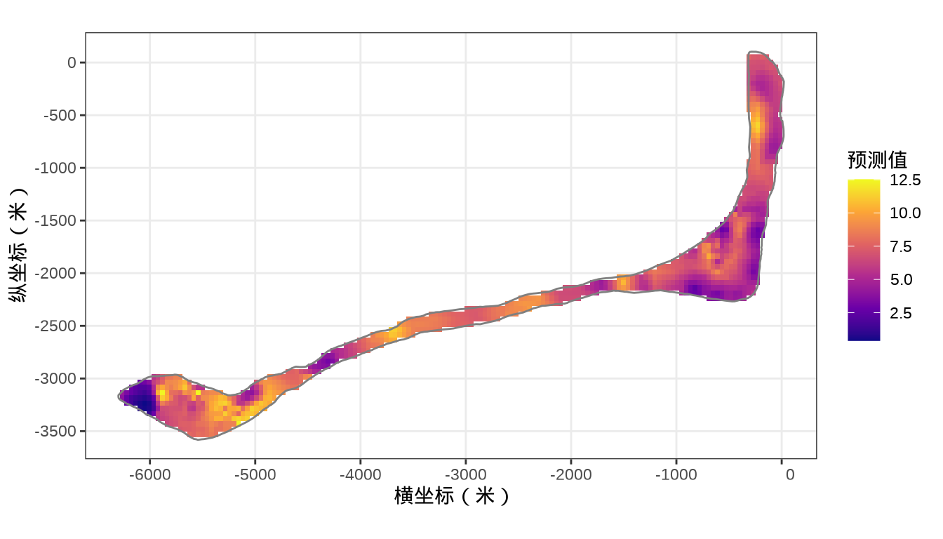
rongelap_stars <- st_crop(x = rongelap_grid_stars, y = rongelap_coastline_sfp)最后,将岛上各个格点的核辐射强度绘制出来,给出全岛核辐射强度的空间分布。
代码
37.2.2 cmdstanr
FRK 包 (Sainsbury-Dale, Zammit-Mangion, 和 Cressie 2022)(Fixed Rank Kriging,固定秩克里金) 可对有一定规模的(时空)空间区域数据和点参考数据集建模,响应变量的分布从高斯分布扩展到指数族,放在(时空)空间广义线性混合效应模型的框架下统一建模。然而,不支持带漂移项的泊松分布。
brms 包支持一大类贝叶斯统计模型,但是对高斯过程建模十分低效,当遇到有一定规模的数据,建模是不可行的,因为经过对 brms 包生成的模型代码的分析,发现它采用潜变量高斯过程(latent variable GP)模型,这也是采样效率低下的一个关键因素。
当设置 \(k = 5\) 时,用 5 个基函数来近似高斯过程,编译完成后,采样速度很快,但是结果不可靠,采样过程中的问题很多。当将横、纵坐标值同时缩小 6000 倍,采样效率并未得到改善。当设置 \(k = 15\) 时,运行时间明显增加,采样过程的诊断结果类似 \(k = 5\) 的情况,还是不可靠。截止写作时间,函数 gp() 的参数 cov 只能取指数二次核函数(exponentiated-quadratic kernel) 。说明 brms 包不适合处理含高斯过程的模型。
实际上,Stan 没有现成的有效算法或扩展包做有规模的高斯过程建模,详见 Bob Carpenter 在 2023 年 Stan 大会的报告,因此,必须采用一些近似方法,通过 Stan 编码实现。接下来,分别手动实现低秩和基样条两种方法近似边际高斯过程(marginal likelihood GP)(Rasmussen 和 Williams 2006),用 Stan 编码模型。代码文件分别是 rongelap_poisson_lr.stan 和 rongelap_poisson_splines.stan 。
37.2.3 GINLA
mgcv 包的函数 ginla() 实现简化版的 Integrated Nested Laplace Approximation, INLA (Simon N. Wood 2019)。
rongelap_gam <- gam(
  counts ~ s(cX, cY, bs = "gp", k = 50), offset = log(time),
  data = rongelap, family = poisson(link = "log"), fit = FALSE
)
# 简化版 INLA
rongelap_ginla <- ginla(G = rongelap_gam)
str(rongelap_ginla)
#> List of 2
#> $ density: num [1:50, 1:100] 2.49e-01 9.03e-06 3.51e-06 1.97e-06 1.17e-06 ...
#> $ beta : num [1:50, 1:100] 1.97 -676.61 -572.67 4720.77 240.12 ...其中, \(k = 50\) 表示 49 个样条参数,每个参数的分布对应有 100 个采样点,另外,截距项的边际后验概率密度分布如下:
plot(
  rongelap_ginla$beta[1, ], rongelap_ginla$density[1, ],
  type = "l", xlab = "截距项", ylab = "概率密度"
)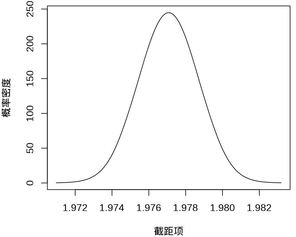
不难看出,截距项在 1.976 至 1.978 之间,50个参数的最大后验估计分别如下:
#>  [1]  1.977019e+00 -5.124099e+02  5.461183e+03  1.515296e+03 -2.822166e+03
#>  [6] -1.598371e+04 -6.417855e+03  1.938122e+02 -4.270878e+03  3.769951e+03
#> [11] -1.002035e+04  1.914717e+03 -9.721572e+03 -3.794461e+04 -1.401549e+04
#> [16] -5.376582e+04 -1.585899e+04 -2.338235e+04  6.239053e+04 -3.574500e+02
#> [21] -4.587927e+04  1.723604e+04 -4.514781e+03  9.184026e-02  3.496526e-01
#> [26] -1.477406e+02  4.585057e+03  9.153647e+03  1.929387e+04 -1.116512e+04
#> [31] -1.166149e+04  8.079451e+02  3.627369e+03 -9.835680e+03  1.357777e+04
#> [36]  1.487742e+04  3.880562e+04 -1.708858e+03  2.775844e+04  2.527415e+04
#> [41] -3.932957e+04  3.548123e+04 -1.116341e+04  1.630910e+04 -9.789381e+02
#> [46] -2.011250e+04  2.699657e+04 -4.744393e+04  2.753347e+04  2.834356e+04
37.2.4 INLA
接下来,介绍完整版的近似贝叶斯推断方法 INLA — 集成嵌套拉普拉斯近似 (Integrated Nested Laplace Approximations,简称 INLA) (Rue, Martino, 和 Chopin 2009)。根据研究区域的边界构造非凸的内外边界,处理边界效应。
library(INLA)
library(splancs)
# 构造非凸的边界
boundary <- list(
  inla.nonconvex.hull(
    points = as.matrix(rongelap_coastline[,c("cX", "cY")]),
    convex = 100, concave = 150, resolution = 100),
  inla.nonconvex.hull(
    points = as.matrix(rongelap_coastline[,c("cX", "cY")]),
    convex = 200, concave = 200, resolution = 200)
)
根据研究区域的情况构造网格,边界内部三角网格最大边长为 300,边界外部最大边长为 600,边界外凸出距离为 100 米。
构建 SPDE,指定自协方差函数为指数型,则 \(\nu = 1/2\) ,因是二维平面,则 \(d = 2\) ,根据 \(\alpha = \nu + d/2\) ,从而 alpha = 3/2 。
生成 SPDE 模型的指标集,也是随机效应部分。
#>       s s.group  s.repl
#>     691     691     691
投影矩阵,三角网格和采样点坐标之间的投影。观测数据 rongelap 和未采样待预测的位置数据 rongelap_grid_df
# 观测位置投影到三角网格上
A <- inla.spde.make.A(mesh = mesh, loc = as.matrix(rongelap[, c("cX", "cY")]) )
# 预测位置投影到三角网格上
coop <- as.matrix(rongelap_grid_df[, c("cX", "cY")])
Ap <- inla.spde.make.A(mesh = mesh, loc = coop)
# 1612 个预测位置
dim(Ap)
#> [1] 1612 691准备观测数据和预测位置,构造一个 INLA 可以使用的数据栈 Data Stack。
# 在采样点的位置上估计 estimation stk.e
stk.e <- inla.stack(
  tag = "est",
  data = list(y = rongelap$counts, E = rongelap$time),
  A = list(rep(1, 157), A),
  effects = list(data.frame(b0 = 1), s = indexs)
)

# 在新生成的位置上预测 prediction stk.p
stk.p <- inla.stack(
  tag = "pred",
  data = list(y = NA, E = NA),
  A = list(rep(1, 1612), Ap),
  effects = list(data.frame(b0 = 1), s = indexs)
)

# 合并数据 stk.full has stk.e and stk.p
stk.full <- inla.stack(stk.e, stk.p)
指定响应变量与漂移项、联系函数、模型公式。
# 精简输出
inla.setOption(short.summary = TRUE)
# 模型拟合
res <- inla(formula = y ~ 0 + b0 + f(s, model = spde),
  data = inla.stack.data(stk.full),
  E = E, # E 已知漂移项
  control.family = list(link = "log"),
  control.predictor = list(
    compute = TRUE,
    link = 1, # 与 control.family 联系函数相同
    A = inla.stack.A(stk.full)
  ),
  control.compute = list(
    cpo = TRUE,
    waic = TRUE, # WAIC 统计量 通用信息准则
    dic = TRUE   # DIC 统计量 偏差信息准则
  ),
  family = "poisson"
)
# 模型输出
summary(res)
#> Fixed effects:
#> mean sd 0.025quant 0.5quant 0.975quant mode kld
#> b0 1.828 0.061 1.706 1.828 1.948 1.828 0
#>
#> Model hyperparameters:
#> mean sd 0.025quant 0.5quant 0.975quant mode
#> Theta1 for s 2.00 0.062 1.88 2.00 2.12 2.00
#> Theta2 for s -4.85 0.130 -5.11 -4.85 -4.59 -4.85
#>
#> Deviance Information Criterion (DIC) ...............: 1834.57
#> Deviance Information Criterion (DIC, saturated) ....: 314.90
#> Effective number of parameters .....................: 156.46
#>
#> Watanabe-Akaike information criterion (WAIC) ...: 1789.32
#> Effective number of parameters .................: 80.06
#>
#> is computedkld表示 Kullback-Leibler divergence (KLD) 它的值描述标准高斯分布与 Simplified Laplace Approximation 之间的差别,值越小越表示拉普拉斯的近似效果好。DIC 和 WAIC 指标都是评估模型预测表现的。另外,还有两个量计算出来了,但是没有显示,分别是 CPO 和 PIT 。CPO 表示 Conditional Predictive Ordinate (CPO),PIT 表示 Probability Integral Transforms (PIT) 。
固定效应(截距)和超参数部分
#>        mean         sd 0.025quant 0.5quant 0.975quant     mode          kld
#> b0 1.828027 0.06147354 1.706422 1.828284 1.948169 1.828279 1.782548e-08#> mean sd 0.025quant 0.5quant 0.975quant mode
#> Theta1 for s 2.000684 0.06235057 1.876512 2.001169 2.122006 2.003209
#> Theta2 for s -4.851258 0.12973411 -5.105061 -4.851807 -4.594252 -4.854094提取预测数据,并整理数据。
# 预测值对应的指标集合
index <- inla.stack.index(stk.full, tag = "pred")$data
# 提取预测结果,后验均值
# pred_mean <- res$summary.fitted.values[index, "mean"]
# 95% 预测下限
# pred_ll <- res$summary.fitted.values[index, "0.025quant"]
# 95% 预测上限
# pred_ul <- res$summary.fitted.values[index, "0.975quant"]
# 整理数据
rongelap_grid_df$ypred <- res$summary.fitted.values[index, "mean"]
# 预测值数据
rongelap_grid_sf <- st_as_sf(rongelap_grid_df, coords = c("cX", "cY"), dim = "XY")
rongelap_grid_stars <- st_rasterize(rongelap_grid_sf, nx = 150, ny = 75)
rongelap_stars <- st_crop(x = rongelap_grid_stars, y = rongelap_coastline_sfp)
最后,类似之前 mgcv 建模的最后一步,将 INLA 的预测结果绘制出来。
37.3 案例:城市土壤重金属污染
介绍多元地统计(Multivariate geostatistics)建模分析与 INLA 实现。分析某城市地表土壤重金属污染情况,找到污染最严重的地方,即寻找重金属污染的源头。
city_df <- readRDS(file = "data/cumcm2011A.rds")
library(sf)
city_sf <- st_as_sf(city_df, coords = c("x(m)", "y(m)"), dim = "XY")
city_sf
#> Simple feature collection with 319 features and 12 fields
#> Geometry type: POINT
#> Dimension: XY
#> Bounding box: xmin: 0 ymin: 0 xmax: 28654 ymax: 18449
#> CRS: NA
#> First 10 features:
#> 编号 功能区 海拔(m) 功能区名称 As (μg/g) Cd (ng/g) Cr (μg/g) Cu (μg/g)
#> 1 1 4 5 交通区 7.84 153.8 44.31 20.56
#> 2 2 4 11 交通区 5.93 146.2 45.05 22.51
#> 3 3 4 28 交通区 4.90 439.2 29.07 64.56
#> 4 4 2 4 工业区 6.56 223.9 40.08 25.17
#> 5 5 4 12 交通区 6.35 525.2 59.35 117.53
#> 6 6 2 6 工业区 14.08 1092.9 67.96 308.61
#> 7 7 4 15 交通区 8.94 269.8 95.83 44.81
#> 8 8 2 7 工业区 9.62 1066.2 285.58 2528.48
#> 9 9 4 22 交通区 7.41 1123.9 88.17 151.64
#> 10 10 4 7 交通区 8.72 267.1 65.56 29.65
#> Hg (ng/g) Ni (μg/g) Pb (μg/g) Zn (μg/g) geometry
#> 1 266 18.2 35.38 72.35 POINT (74 781)
#> 2 86 17.2 36.18 94.59 POINT (1373 731)
#> 3 109 10.6 74.32 218.37 POINT (1321 1791)
#> 4 950 15.4 32.28 117.35 POINT (0 1787)
#> 5 800 20.2 169.96 726.02 POINT (1049 2127)
#> 6 1040 28.2 434.80 966.73 POINT (1647 2728)
#> 7 121 17.8 62.91 166.73 POINT (2883 3617)
#> 8 13500 41.7 381.64 1417.86 POINT (2383 3692)
#> 9 16000 25.8 172.36 926.84 POINT (2708 2295)
#> 10 63 21.7 36.94 100.41 POINT (2933 1767)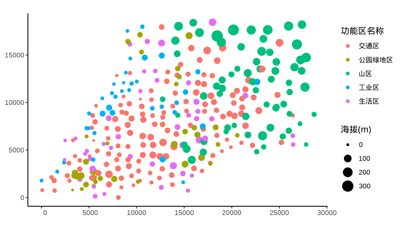
类似 章节 37.2.1 ,下面根据数据构造城市边界以及对城市区域划分,以便预测城市中其它地方的重金属浓度。
# 由点构造多边形
city_sfp <- st_cast(st_combine(st_geometry(city_sf)), "POLYGON")
# 由点构造凸包
city_hull <- st_convex_hull(st_geometry(city_sfp))
# 添加缓冲区作为城市边界
city_buffer <- st_buffer(city_hull, dist = 1000)
# 构造带边界约束的网格
city_grid <- st_make_grid(city_buffer, n = c(150, 75))
# 将 sfc 类型转化为 sf 类型
city_grid <- st_as_sf(city_grid)
city_buffer <- st_as_sf(city_buffer)
city_grid <- city_grid[city_buffer, op = st_intersects]
# 计算网格中心点坐标
city_grid_centroid <- st_centroid(city_grid)
# 共计 8494 个预测点
city_grid_df <- as.data.frame(st_coordinates(city_grid_centroid))
城市边界线
ggplot() +
  geom_sf(data = city_sf, aes(color = `功能区名称`, size = `海拔(m)`)) +
  geom_sf(data = city_hull, fill = NA) +
  geom_sf(data = city_buffer, fill = NA) +
  theme_classic()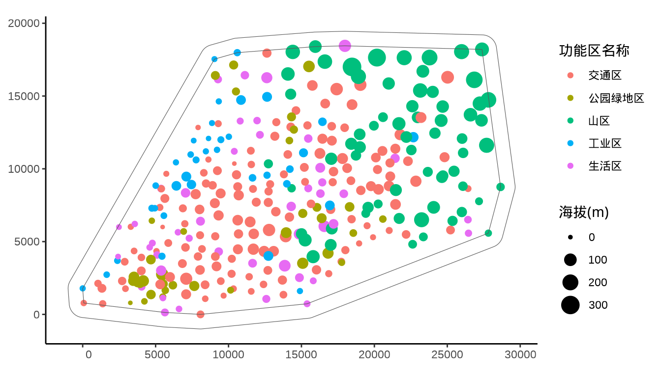
根据横、纵坐标和海拔数据,通过高斯过程回归(当然可以用其他办法,这里仅做示意)拟合获得城市其他位置的海拔,绘制等高线图,一目了然地获得城市地形信息。
library(mgcv)
# 提取部分数据
city_topo <- subset(city_df, select = c("x(m)", "y(m)", "海拔(m)"))
colnames(city_topo) <- c("x", "y", "z")
# 高斯过程拟合
fit_city_mgcv <- gam(z ~ s(x, y, bs = "gp", k = 50),
  data = city_topo, family = gaussian(link = "identity")
)
# 绘制等高线图
# vis.gam(fit_city_mgcv, color = "cm", plot.type = "contour", n.grid = 50)
colnames(city_grid_df) <- c("x", "y")
# 预测
city_grid_df$zpred <- as.vector(predict(fit_city_mgcv, newdata = city_grid_df, type = "response"))
# 转化数据
city_grid_sf <- st_as_sf(city_grid_df, coords = c("x", "y"), dim = "XY")
library(stars)
city_stars <- st_rasterize(city_grid_sf, nx = 150, ny = 75)ggplot() +
geom_stars(data = city_stars, aes(fill = zpred), na.action = na.omit) +
geom_sf(data = city_buffer, fill = NA, color = "gray50", linewidth = .5) +
scale_fill_viridis_c(option = "C") +
theme_bw() +
labs(x = "横坐标(米)", y = "纵坐标(米)", fill = "海拔(米)")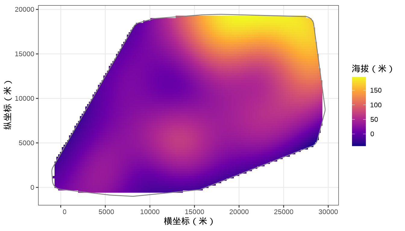
library(ggplot2)
ggplot(data = city_sf) +
geom_sf(aes(color = `功能区名称`, size = `As (μg/g)`)) +
theme_classic()
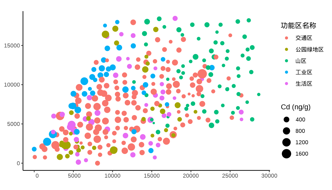
ggplot(data = city_sf) +
geom_sf(aes(color = `功能区名称`, size = `Cd (ng/g)`)) +
theme_classic()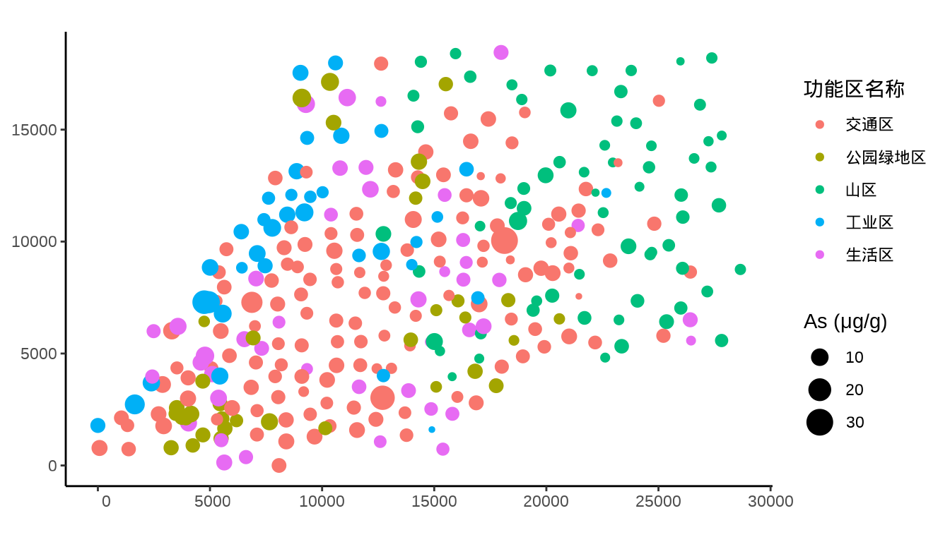
为了便于建模,对数据做标准化处理。
# 根据背景值将各个重金属浓度列进行转化
city_sf <- within(city_sf, {
`As (μg/g)` <- (`As (μg/g)` - 3.6) / 0.9
`Cd (ng/g)` <- (`Cd (ng/g)` - 130) / 30
`Cr (μg/g)` <- (`Cr (μg/g)` - 31) / 9
`Cu (μg/g)` <- (`Cu (μg/g)` - 13.2) / 3.6
`Hg (ng/g)` <- (`Hg (ng/g)` - 35) / 8
`Ni (μg/g)` <- (`Ni (μg/g)` - 12.3) / 3.8
`Pb (μg/g)` <- (`Pb (μg/g)` - 31) / 6
`Zn (μg/g)` <- (`Zn (μg/g)` - 69) / 14
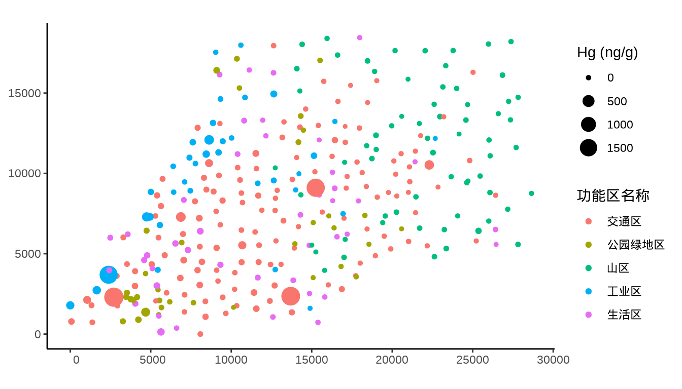
})当我们逐一检查各个重金属的浓度分布时,发现重金属汞 Hg 在四个地方的浓度极高,暗示着如果数据采集没有问题,那么这几个地方很可能是污染源。
37.3.1 mgcv
mgcv 包用于多元空间模型中样条参数估计和选择 (Simon N. Wood, Pya, 和 Säfken 2016)。
37.3.2 INLA
INLA 包用于多元空间模型的贝叶斯推断 (Palmí-Perales 等 2022) 。