38 高斯过程回归
\[ \def\bm#1{{\boldsymbol #1}} \]
本章主要内容分三大块,分别是多元正态分布、二维高斯过程和高斯过程回归。根据高斯过程的定义,我们知道多元正态分布和高斯过程有紧密的联系,首先介绍多元正态分布的定义、随机数模拟和分布拟合。二维高斯过程很有代表性,常用于空间统计中,而一维高斯过程常用于时间序列分析中,因而,介绍高斯过程的定义,二维高斯过程的模拟和参数拟合。在后续的高斯过程回归中,以朗格拉普岛的核辐射数据为例,建立泊松空间广义线性混合效应模型(响应变量非高斯的高斯过程回归模型),随机过程看作一组存在相关性的随机变量,这一组随机变量视为模型中的随机效应。
38.1 多元正态分布
设随机向量 \(\bm{X} = (X_1, X_2, \cdots, X_p)^{\top}\) 服从多元正态分布 \(\mathrm{MVN}(\bm{\mu}, \Sigma)\) ,其联合密度函数如下
\[ \begin{aligned} p(\boldsymbol x) = (2\pi)^{-\frac{p}{2}} |\Sigma|^{-\frac12} \exp\left\{ -\frac12 (\boldsymbol x - \boldsymbol \mu)^T \Sigma^{-1} (\boldsymbol x - \boldsymbol \mu) \right\}, \ \boldsymbol x \in \mathbb{R}^p \end{aligned} \]
其中,协方差矩阵 \(\Sigma\) 是正定的,其 Cholesky 分解为 \(\Sigma = CC^{\top}\) ,这里 \(C\) 为下三角矩阵。设 \(\bm{Z} = (Z_1, Z_2, \cdots, Z_p)^{\top}\) 服从 \(p\) 元标准正态分布 \(\mathrm{MVN}(\bm{0}, I)\) ,则 \(\bm{X} = \bm{\mu} + C\bm{Z}\) 服从多元正态分布 \(\mathrm{MVN}(\bm{\mu}, \Sigma)\) 。
38.1.1 多元正态分布模拟
可以用 Stan 函数 multi_normal_cholesky_rng 生成随机数模拟多元正态分布。
data {
  int<lower=1> N;
  int<lower=1> D;
  vector[D] mu;
  matrix[D, D] Sigma;
}
transformed data {
  matrix[D, D] L_K = cholesky_decompose(Sigma);
}
parameters {
}
model {
}
generated quantities {
  array[N] vector[D] yhat;
  for (n in 1:N){
    yhat[n] = multi_normal_cholesky_rng(mu, L_K);
  }
}
上述代码块可以同时模拟多组服从多元正态分布的随机数。其中,参数块 parameters 和模型块 model 是空白的,这是因为模拟随机数不涉及模型推断,只是采样。核心部分 generated quantities 代码块负责生成随机数。
抽样生成 1000 个服从二元正态分布的随机数。
simu_multi_normal <- mod_multi_normal$sample(
  data = multi_normal_d,
  iter_warmup = 500,    # 每条链预处理迭代次数
  iter_sampling = 1000, # 样本量
  chains = 1,           # 马尔科夫链的数目
  parallel_chains = 1,  # 指定 CPU 核心数,可以给每条链分配一个
  threads_per_chain = 1, # 每条链设置一个线程
  show_messages = FALSE, # 不显示迭代的中间过程
  refresh = 0,        # 不显示采样的进度
  fixed_param = TRUE, # 固定参数
  output_dir = "data-raw/",
  seed = 20232023     # 设置随机数种子,不要使用 set.seed() 函数
)
值得注意,这里,不需要设置参数初始值,但要设置 fixed_param = TRUE,表示根据模型生成模拟数据。
# A draws_array: 1000 iterations, 1 chains, and 2 variables
, , variable = yhat[1,1]

         chain
iteration   1
        1 2.6
        2 5.3
        3 1.4
        4 3.1
        5 7.6

, , variable = yhat[1,2]

         chain
iteration    1
        1 0.65
        2 3.70
        3 4.36
        4 1.85
        5 2.32

# ... with 995 more iterations
# A tibble: 2 × 10
variable mean median sd mad q5 q95 rhat ess_bulk ess_tail
<chr> <dbl> <dbl> <dbl> <dbl> <dbl> <dbl> <dbl> <dbl> <dbl>
1 yhat[1,1] 3.076 2.979 2.038 1.916 -0.3290 6.535 1.001 1140. 1023.
2 yhat[1,2] 1.990 1.964 1.018 0.9765 0.2323 3.680 1.002 966.5 982.1以生成第一个服从二元正态分布的随机数(样本点)为例,这个随机数是通过采样获得的,采样过程中产生一个采样序列,采样序列的轨迹和分布如下:
library(ggplot2)
library(bayesplot)
mcmc_trace(simu_multi_normal$draws(c("yhat[1,1]", "yhat[1,2]")),
  facet_args = list(
    labeller = ggplot2::label_parsed,
    strip.position = "top", ncol = 1
  )
) + theme_bw(base_size = 12)

mcmc_dens(simu_multi_normal$draws(c("yhat[1,1]", "yhat[1,2]")),
  facet_args = list(
    labeller = ggplot2::label_parsed,
    strip.position = "top", ncol = 1
  )
) + theme_bw(base_size = 12)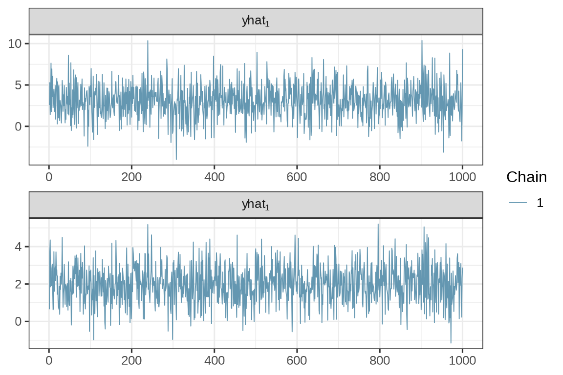
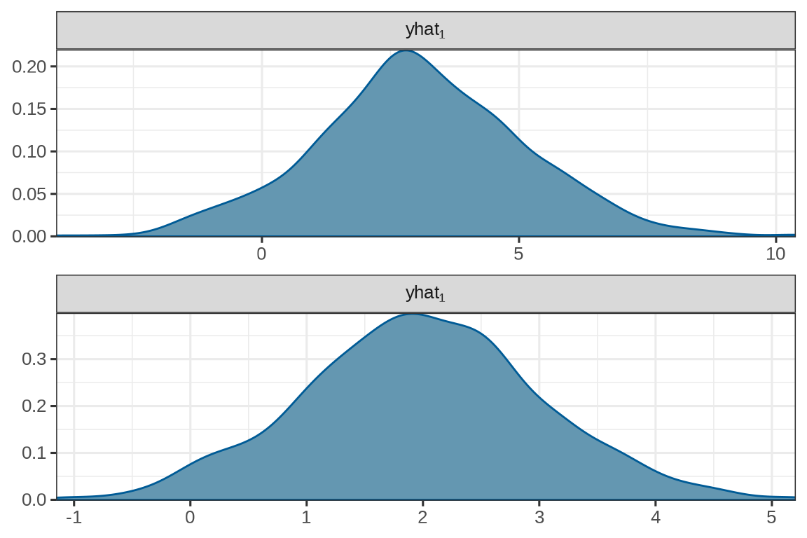
这就是一组来自二元正态分布的随机数。
mcmc_scatter(simu_multi_normal$draws(c("yhat[1,1]", "yhat[1,2]"))) +
  theme_bw(base_size = 12) +
  labs(x = expression(x[1]), y = expression(x[2]))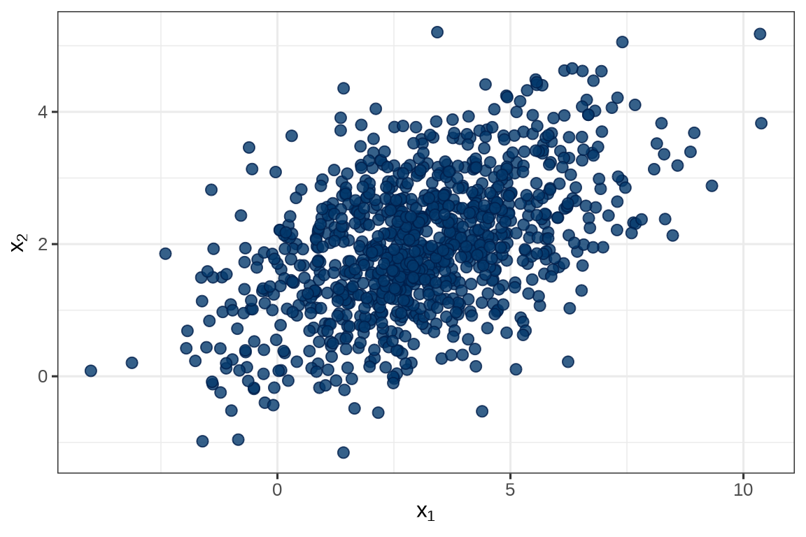
提取采样数据,整理成矩阵。
38.1.2 多元正态分布拟合
一般地,协方差矩阵的 Cholesky 分解的矩阵表示如下:
\[ \begin{aligned} \Sigma &= \begin{bmatrix} \sigma^2_1 & \rho_{12}\sigma_1\sigma_2 & \rho_{13}\sigma_1\sigma_3 \\ \rho_{12}\sigma_1\sigma_2 & \sigma_2^2 & \rho_{23}\sigma_2\sigma_3 \\ \rho_{13}\sigma_1\sigma_3 & \rho_{23}\sigma_2\sigma_3 & \sigma_3^2 \end{bmatrix} \\ & = \begin{bmatrix} \sigma_1 & 0 & 0 \\ 0 & \sigma_2 & 0 \\ 0 & 0 & \sigma_3 \end{bmatrix} \underbrace{ \begin{bmatrix} 1 & \rho_{12} & \rho_{13} \\ \rho_{12} & 1 & \rho_{23} \\ \rho_{13} & \rho_{23} & 1 \end{bmatrix} }_{R} \begin{bmatrix} \sigma_1 & 0 & 0 \\ 0 & \sigma_2 & 0 \\ 0 & 0 & \sigma_3 \end{bmatrix} \\ & = \begin{bmatrix} \sigma_1 & 0 & 0 \\ 0 & \sigma_2 & 0 \\ 0 & 0 & \sigma_3 \end{bmatrix} \underbrace{L_u L_u^{\top}}_{R} \begin{bmatrix} \sigma_1 & 0 & 0 \\ 0 & \sigma_2 & 0 \\ 0 & 0 & \sigma_3 \end{bmatrix} \end{aligned} \]
data {
  int<lower=1> N; // number of observations
  int<lower=1> K; // dimension of observations
  array[N] vector[K] y; // observations: a list of N vectors (each has K elements)
}
parameters {
  vector[K] mu;
  cholesky_factor_corr[K] Lcorr; // cholesky factor (L_u matrix for R)
  vector<lower=0>[K] sigma;
}
transformed parameters {
  corr_matrix[K] R; // correlation matrix
  cov_matrix[K] Sigma; // VCV matrix
  R = multiply_lower_tri_self_transpose(Lcorr); // R = Lcorr * Lcorr'
  Sigma = quad_form_diag(R, sigma); // quad_form_diag: diag_matrix(sig) * R * diag_matrix(sig)
}
model {
  sigma ~ cauchy(0, 5); // prior for sigma
  Lcorr ~ lkj_corr_cholesky(2.0); // prior for cholesky factor of a correlation matrix
  y ~ multi_normal(mu, Sigma);
}
代码中, 核心部分是关于多元正态分布的协方差矩阵的参数化,先将协方差矩阵中的方差和相关矩阵剥离,然后利用 Cholesky 分解将相关矩阵分解。在 Stan 里,这是一套高效的组合。
类型
cholesky_factor_corr表示相关矩阵的 Cholesky 分解后的矩阵 \(L_u\)类型
corr_matrix表示相关矩阵 \(R\) 。类型
cov_matrix表示协方差矩阵 \(\Sigma\) 。函数
lkj_corr_cholesky为相关矩阵 Cholesky 分解后的矩阵 \(L_u\) 服从的分布,详见 Cholesky LKJ correlation distribution。函数名中的lkj是以三个人的人名的首字母命名的 Lewandowski, Kurowicka, and Joe 2009。函数
multiply_lower_tri_self_transpose为下三角矩阵与它的转置的乘积,详见 Correlation Matrix Distributions。函数
multi_normal为多元正态分布的抽样语句,详见 Multivariate normal distribution。
矩阵 \(L_u\) 是相关矩阵 \(R\) 的 Cholesky 分解的结果,在贝叶斯框架内,参数都是随机的,相关矩阵是一个随机矩阵,矩阵 \(L_u\) 是一个随机矩阵,它的分布用 Stan 代码表示为如下:
LKJ 分布有一个参数 \(\eta\) ,此处 \(\eta = 2\) ,意味着变量之间的相关性较弱,LKJ 分布的概率密度函数正比于相关矩阵的行列式的 \(\eta-1\) 次幂 \((\det{R})^{\eta-1}\),LKJ 分布的详细说明见Lewandowski-Kurowicka-Joe (LKJ) distribution。
有了上面的背景知识,下面先在 R 环境中模拟一组来自多元正态分布的样本。
根据 1000 个样本点,估计多元正态分布的均值参数和方差协方差参数。
# 来自多元正态分布的一组观测数据
multi_normal_chol_d <- list(
  N = 1000, # 样本量
  K = 3,    # 三维
  y = dat
)
# 编译多元正态分布模型
mod_multi_normal_chol <- cmdstan_model(
  stan_file = "code/multi_normal_fitted.stan",
  compile = TRUE, cpp_options = list(stan_threads = TRUE)
)
# 拟合多元正态分布模型
fit_multi_normal <- mod_multi_normal_chol$sample(
  data = multi_normal_chol_d,
  iter_warmup = 500,    # 每条链预处理迭代次数
  iter_sampling = 1000, # 每条链采样次数
  chains = 2,           # 马尔科夫链的数目
  parallel_chains = 1,  # 指定 CPU 核心数
  threads_per_chain = 1,  # 每条链设置一个线程
  show_messages = FALSE,  # 不显示迭代的中间过程
  refresh = 0,            # 不显示采样的进度
  output_dir = "data-raw/",
  seed = 20232023     # 设置随机数种子
)
均值向量 \(\bm{\mu}\) 和协方差矩阵 \(\Sigma\) 估计结果如下:
# A tibble: 12 × 10
variable mean median sd mad q5 q95 rhat ess_bulk ess_tail
<chr> <dbl> <dbl> <dbl> <dbl> <dbl> <dbl> <dbl> <dbl> <dbl>
1 mu[1] 1.02 1.02 0.0162 0.0154 0.999 1.05 1.00 1605. 1250.
2 mu[2] 2.00 2.00 0.0385 0.0386 1.93 2.06 1.00 1300. 1138.
3 mu[3] -4.86 -4.86 0.0703 0.0724 -4.98 -4.75 1.00 1737. 1549.
4 Sigma[1,1] 0.250 0.249 0.0110 0.0108 0.231 0.268 1.00 1847. 1336.
5 Sigma[2,1] 0.427 0.426 0.0235 0.0234 0.388 0.466 1.00 1507. 1261.
6 Sigma[3,1] 0.210 0.209 0.0361 0.0363 0.151 0.271 1.00 1472. 1202.
7 Sigma[1,2] 0.427 0.426 0.0235 0.0234 0.388 0.466 1.00 1507. 1261.
8 Sigma[2,2] 1.47 1.47 0.0649 0.0635 1.37 1.58 1.01 1506. 1265.
9 Sigma[3,2] -1.41 -1.41 0.0955 0.0957 -1.57 -1.26 1.00 1643. 1572.
10 Sigma[1,3] 0.210 0.209 0.0361 0.0363 0.151 0.271 1.00 1472. 1202.
11 Sigma[2,3] -1.41 -1.41 0.0955 0.0957 -1.57 -1.26 1.00 1643. 1572.
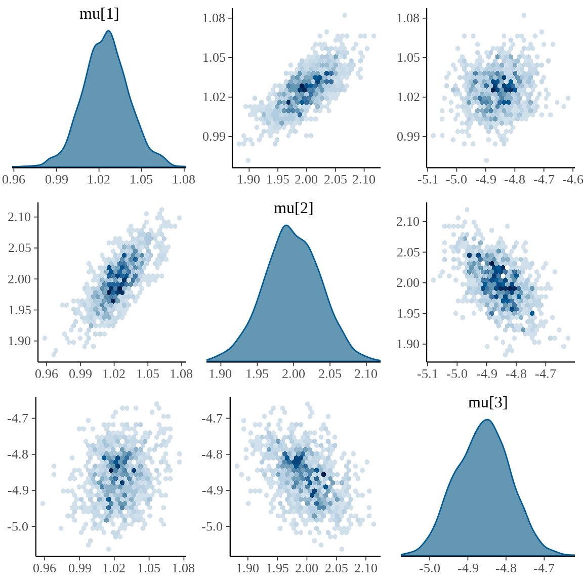
12 Sigma[3,3] 5.28 5.27 0.225 0.221 4.92 5.67 1.00 1605. 1603.均值向量 \(\bm{\mu} = (\mu_1,\mu_2,\mu_3)^{\top}\) 各个分量及其两两相关性,如下图所示。
38.2 二维高斯过程
高斯过程定义
38.2.1 二维高斯过程模拟
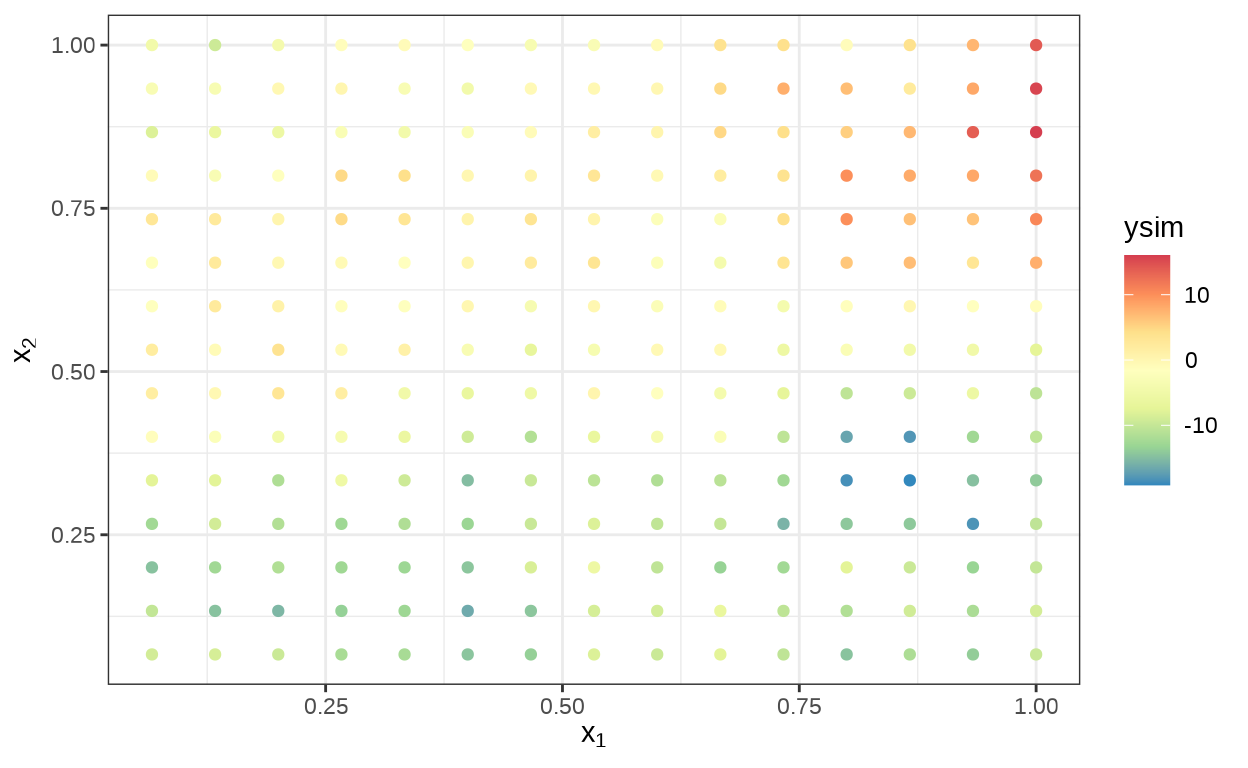
二维高斯过程 \(\mathcal{S}\) 的均值向量为 0 向量,自协方差函数为指数型,如下
\[ \mathsf{Cov}\{S(x_i), S(x_j)\} = \sigma^2 \exp\big( -\frac{\|x_i -x_j\|_{2}}{\phi} \big) \]
其中,不妨设参数 \(\sigma = 10, \phi = 1\) 。模拟高斯过程的 Stan 代码如下
data {
  int<lower=1> N;
  int<lower=1> D;
  array[N] vector[D] X;
  vector[N] mu;
  real<lower=0> sigma;
  real<lower=0> phi;
}
transformed data {
  real delta = 1e-9;
  matrix[N, N] L;
  matrix[N, N] K = gp_exponential_cov(X, sigma, phi) + diag_matrix(rep_vector(delta, N));
  L = cholesky_decompose(K);
}
parameters {
  vector[N] eta;
}
model {
  eta ~ std_normal();
}
generated quantities {
  vector[N] y;
  y = mu + L * eta;
}
在二维规则网格上采样,采样点数量为 225。
模拟 1 个样本,因为是模拟数据,不需要设置多条链。
fit_multi_normal_gp <- mod_gaussian_process_simu$sample(
  data = gaussian_process_d,
  iter_warmup = 500,       # 每条链预处理迭代次数
  iter_sampling = 1000,    # 样本量
  chains = 1,              # 马尔科夫链的数目
  parallel_chains = 1,    # 指定 CPU 核心数
  threads_per_chain = 1,  # 每条链设置一个线程
  show_messages = FALSE,  # 不显示迭代的中间过程
  refresh = 0,            # 不显示采样的进度
  output_dir = "data-raw/",
  seed = 20232023         # 设置随机数种子
)
位置 1 和 2 处的随机变量的迭代轨迹,均值为 0 ,标准差 10 左右。
mcmc_trace(fit_multi_normal_gp$draws(c("y[1]", "y[2]")),
  facet_args = list(
    labeller = ggplot2::label_parsed,
    strip.position = "top", ncol = 1
  )
) + theme_bw(base_size = 12)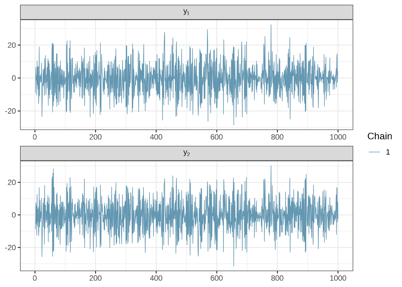
位置 1 处的随机变量及其分布
y1 <- fit_multi_normal_gp$draws(c("y[1]"), format = "draws_array")
# 合并链条结果
y1_mean <- apply(y1, c(1, 3), mean)
# y[1] 的方差
var(y1_mean)
y[1]
y[1] 100.5436[1] 10.02714100 次迭代获得 100 个样本点,每次迭代采集一个样本点,每个样本点是一个 225 维的向量。
从 100 次迭代中任意提取某一个样本点,比如预采样之后的第一次下迭代的结果,接着整理数据。
绘制二维高斯过程图形。
38.2.2 二维高斯过程拟合
二维高斯过程拟合代码如下
data {
  int<lower=1> N;
  int<lower=1> D;
  array[N] vector[D] x;
  vector[N] y;
}
transformed data {
  real delta = 1e-9;
  vector[N] mu = rep_vector(0, N);
}
parameters {
  real<lower=0> phi;
  real<lower=0> sigma;
}
model {
  matrix[N, N] L_K;
  {
    matrix[N, N] K = gp_exponential_cov(x, sigma, phi) + diag_matrix(rep_vector(delta, N));
    L_K = cholesky_decompose(K);
  }

  phi ~ std_normal();
  sigma ~ std_normal();

  y ~ multi_normal_cholesky(mu, L_K);
}
# 二维高斯过程模型
gaussian_process_d <- list(
D = 2,
N = nrow(sim_gp_data), # 观测记录的条数
x = sim_gp_data[, c("x1", "x2")],
y = sim_gp_data[, "ysim"]
)
nchains <- 2
set.seed(20232023)
# 给每条链设置不同的参数初始值
inits_gaussian_process <- lapply(1:nchains, function(i) {
list(
sigma = runif(1),
phi = runif(1)
)
})
# 编译模型
mod_gaussian_process <- cmdstan_model(
stan_file = "code/gaussian_process_fitted.stan",
compile = TRUE, cpp_options = list(stan_threads = TRUE)
)
# 拟合二维高斯过程
fit_gaussian_process <- mod_gaussian_process$sample(
data = gaussian_process_d, # 观测数据
init = inits_gaussian_process, # 迭代初值
iter_warmup = 1000, # 每条链预处理迭代次数
iter_sampling = 2000, # 每条链总迭代次数
chains = nchains, # 马尔科夫链的数目
parallel_chains = 2, # 指定 CPU 核心数,可以给每条链分配一个
threads_per_chain = 2, # 每条链设置一个线程
show_messages = FALSE, # 不显示迭代的中间过程
refresh = 0, # 不显示采样的进度
output_dir = "data-raw/",
seed = 20232023 # 设置随机数种子,不要使用 set.seed() 函数
)
# 诊断
fit_gaussian_process$diagnostic_summary()$num_divergent
[1] 0 0
$num_max_treedepth
[1] 0 0
$ebfmi
[1] 1.097944 1.083674输出结果
# A tibble: 3 × 10
  variable     mean   median     sd    mad       q5      q95  rhat ess_bulk
  <chr>       <dbl>    <dbl>  <dbl>  <dbl>    <dbl>    <dbl> <dbl>    <dbl>
1 lp__     -354.    -354.    0.964  0.703  -356.    -353.     1.00    1395.
2 phi         0.308    0.302 0.0503 0.0486    0.235    0.400  1.00    1196.
3 sigma       5.25     5.24  0.389  0.375     4.65     5.94   1.00    1246.
# ℹ 1 more variable: ess_tail <dbl>
38.3 高斯过程回归
38.3.1 模型介绍
朗格拉普岛是位于太平洋上的一个小岛,因美国在比基尼群岛的氢弹核试验受到严重的核辐射影响,数十年之后,科学家登岛采集核辐射强度数据以评估当地居民重返该岛的可能性。朗格拉普岛是一个十分狭长且占地面积只有几平方公里的小岛。
根据 \({}^{137}\mathrm{Cs}\) 放出伽马射线,在 \(n=157\) 个采样点,分别以时间间隔 \(t_i\) 测量辐射量 \(y(x_i)\),建立泊松型空间广义线性混合效应模型(Diggle, Tawn, 和 Moyeed 1998)。
\[ \begin{aligned} \log\{\lambda(x_i)\} & = \beta + S(x_{i})\\ y(x_{i}) &\sim \mathrm{Poisson}\big(t_i\lambda(x_i)\big) \end{aligned} \]
其中,\(\beta\) 表示截距,相当于平均水平,\(\lambda(x_i)\) 表示位置 \(x_i\) 处的辐射强度,\(S(x_{i})\) 表示位置 \(x_i\) 处的空间效应,\(S(x),x \in \mathcal{D} \subset{\mathbb{R}^2}\) 是二维平稳空间高斯过程 \(\mathcal{S}\) 的具体实现。 \(\mathcal{D}\) 表示研究区域,可以理解为朗格拉普岛,它是二维实平面 \(\mathbb{R}^2\) 的子集。
随机过程 \(S(x)\) 的自协方差函数常用的有指数型、幂二次指数型(高斯型)和梅隆型,形式如下:
\[ \begin{aligned} \mathsf{Cov}\{S(x_i), S(x_j)\} &= \sigma^2 \exp\big( -\frac{\|x_i -x_j\|_{2}}{\phi} \big) \\ \mathsf{Cov}\{ S(x_i), S(x_j) \} &= \sigma^2 \exp\big( -\frac{\|x_i -x_j\|_{2}^{2}}{2\phi^2} \big) \\ \mathsf{Cov}\{ S(x_i), S(x_j) \} &= \sigma^2 \frac{2^{1 - \nu}}{\Gamma(\nu)} \left(\sqrt{2\nu}\frac{\|x_i -x_j\|_{2}}{\phi}\right)^{\nu} K_{\nu}\left(\sqrt{2\nu}\frac{\|x_i -x_j\|_{2}}{\phi}\right) \\ K_{\nu}(x) &= \int_{0}^{\infty}\exp(-x \cosh t) \cosh (\nu t) \mathrm{dt} \end{aligned} \]
待估参数:代表方差的 \(\sigma^2\) 和代表范围的 \(\phi\) 。当 \(\nu = 1/2\) 时,梅隆型退化为指数型。
38.3.2 观测数据
# 加载数据
rongelap <- readRDS(file = "data/rongelap.rds")
rongelap_coastline <- readRDS(file = "data/rongelap_coastline.rds")
# 准备输入数据
rongelap_poisson_d <- list(
  N = nrow(rongelap), # 观测记录的条数
  D = 2, # 2 维坐标
  X = rongelap[, c("cX", "cY")] / 6000, # N x 2 矩阵
  y = rongelap$counts, # 响应变量
  offsets = rongelap$time # 漂移项
)
# 准备参数初始化数据
set.seed(20232023)
nchains <- 2 # 2 条迭代链
inits_data_poisson <- lapply(1:nchains, function(i) {
  list(
    beta = rnorm(1),
    sigma = runif(1),
    phi = runif(1),
    lambda = rnorm(157)
  )
})
38.3.3 预测数据
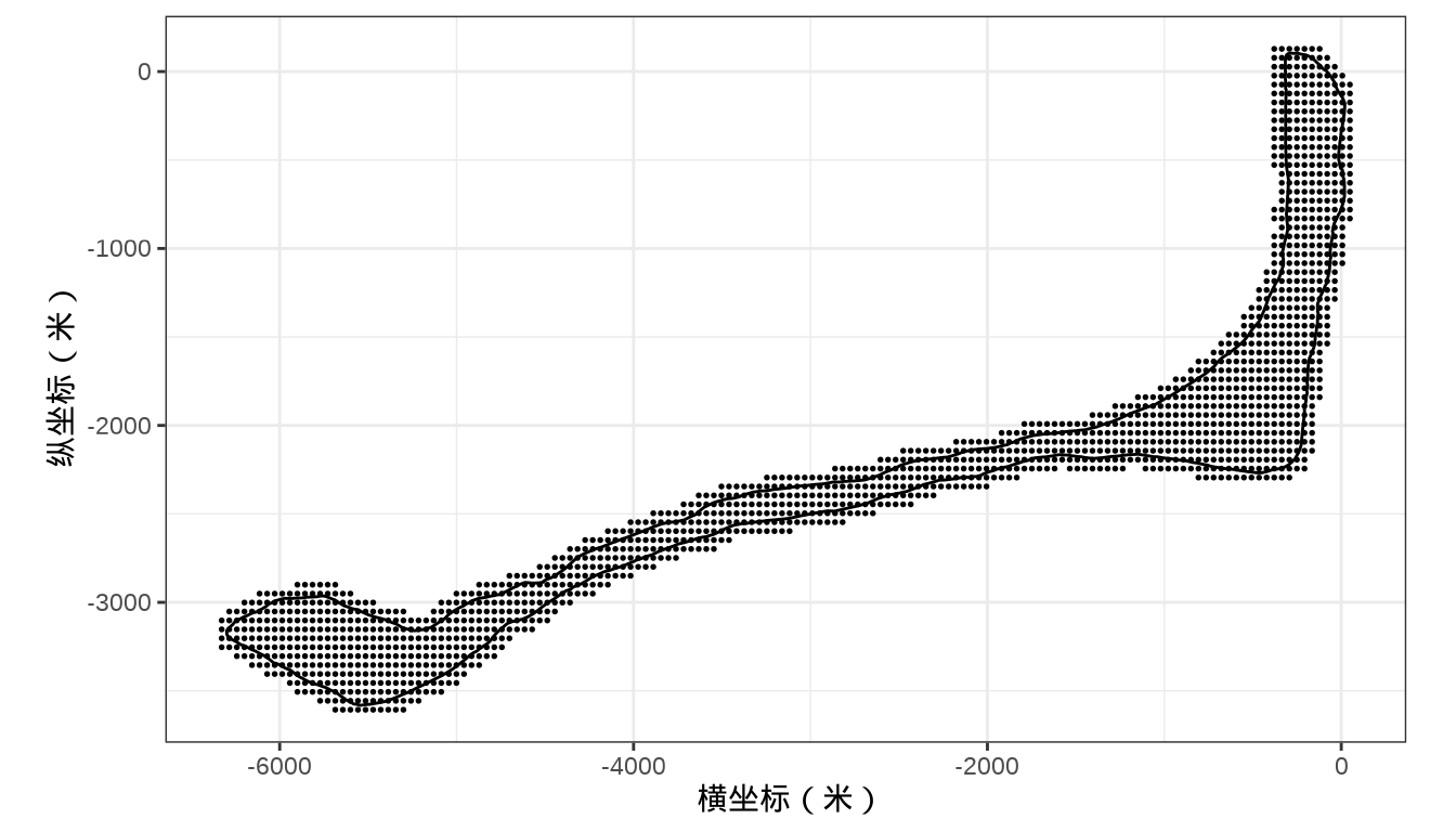
预测未采样的位置的核辐射强度,根据海岸线数据网格化全岛,以格点代表未采样的位置
library(sf)
library(abind)
library(stars)
# 类型转化
rongelap_sf <- st_as_sf(rongelap, coords = c("cX", "cY"), dim = "XY")
rongelap_coastline_sf <- st_as_sf(rongelap_coastline, coords = c("cX", "cY"), dim = "XY")
rongelap_coastline_sfp <- st_cast(st_combine(st_geometry(rongelap_coastline_sf)), "POLYGON")
# 添加缓冲区
rongelap_coastline_buffer <- st_buffer(rongelap_coastline_sfp, dist = 50)
# 构造带边界约束的网格
rongelap_coastline_grid <- st_make_grid(rongelap_coastline_buffer, n = c(150, 75))
# 将 sfc 类型转化为 sf 类型
rongelap_coastline_grid <- st_as_sf(rongelap_coastline_grid)
rongelap_coastline_buffer <- st_as_sf(rongelap_coastline_buffer)
rongelap_grid <- rongelap_coastline_grid[rongelap_coastline_buffer, op = st_intersects]
# 计算网格中心点坐标
rongelap_grid_centroid <- st_centroid(rongelap_grid)
# 共计 1612 个预测点
rongelap_grid_df <- as.data.frame(st_coordinates(rongelap_grid_centroid))
colnames(rongelap_grid_df) <- c("cX", "cY")
未采样的位置 rongelap_grid_df
         cX        cY
1 -5685.942 -3606.997
2 -5643.145 -3606.997
3 -5600.347 -3606.997
4 -5557.549 -3606.997
5 -5514.751 -3606.997
6 -5471.953 -3606.997
朗格拉普岛网格化生成格点
38.3.4 模型编码
指定各个参数 \(\beta,\sigma,\phi\) 的先验分布
\[ \begin{aligned} \beta &\sim \mathrm{std\_normal}(0,1) \\ \sigma &\sim \mathrm{inv\_gamma}(5,5) \\ \phi &\sim \mathrm{half\_std\_normal}(0,1) \\ \bm{\lambda} | \beta,\sigma &\sim \mathrm{multivariate\_normal}(\bm{\beta}, \sigma^2 \Sigma) \\ \bm{y} | \bm{\lambda} &\sim \mathrm{poisson\_log}\big(\log(\text{offsets})+\bm{\lambda}\big) \end{aligned} \]
其中,\(\beta,\sigma,\phi,\Sigma\) 的含义同前,\(\lambda\) 代表辐射强度,\(\mathrm{offsets}\) 代表漂移项,这里是时间段,\(\bm{y}\) 表示观测的辐射粒子数,\(\mathrm{poisson\_log}\) 表示泊松分布的对数参数化,将频率参数 rate 的对数 \(\lambda\) 作为参数,详见 Stan 函数手册中泊松分布的对数函数表示。
data {
  int<lower=1> N;
  int<lower=1> D;
  array[N] vector[D] X;
  array[N] int<lower = 0> y;
  vector[N] offsets;
}
transformed data {
  real delta = 1e-12;
  vector[N] log_offsets = log(offsets);
}
parameters {
  real beta;
  real<lower=0> sigma;
  real<lower=0> phi;
  vector[N] lambda;
}
transformed parameters {
  vector[N] mu = rep_vector(beta, N);
}
model {
  matrix[N, N] L_K;
  {
    matrix[N, N] K = gp_exponential_cov(X, sigma, phi) + diag_matrix(rep_vector(delta, N));
    L_K = cholesky_decompose(K);
  }

  beta ~ std_normal();
  sigma ~ inv_gamma(5, 5);
  phi ~ std_normal();

  lambda ~ multi_normal_cholesky(mu, L_K);
  y ~ poisson_log(log_offsets + lambda);
}
# 编译模型
mod_rongelap_poisson <- cmdstan_model(
stan_file = "code/rongelap_poisson_processes.stan",
compile = TRUE, cpp_options = list(stan_threads = TRUE)
)
# 泊松对数模型
fit_rongelap_poisson <- mod_rongelap_poisson$sample(
data = rongelap_poisson_d, # 观测数据
init = inits_data_poisson, # 迭代初值
iter_warmup = 500, # 每条链预处理迭代次数
iter_sampling = 1000, # 每条链总迭代次数
chains = nchains, # 马尔科夫链的数目
parallel_chains = 2, # 指定 CPU 核心数,可以给每条链分配一个
threads_per_chain = 2, # 每条链设置一个线程
show_messages = FALSE, # 不显示迭代的中间过程
refresh = 0, # 不显示采样的进度
output_dir = "data-raw/",
seed = 20232023
)
# 诊断
fit_rongelap_poisson$diagnostic_summary()$num_divergent
[1] 0 0
$num_max_treedepth
[1] 0 0
$ebfmi
[1] 1.078629 1.048734# 泊松对数模型
fit_rongelap_poisson$summary(
variables = c("lp__", "beta", "sigma", "phi"),
.num_args = list(sigfig = 3, notation = "dec")
)# A tibble: 4 × 10
variable mean median sd mad q5 q95
<chr> <dbl> <dbl> <dbl> <dbl> <dbl> <dbl>
1 lp__ 3402193. 3402190 9.44 14.8 3402180 3402210
2 beta 1.78 1.79 0.139 0.116 1.56 1.97
3 sigma 0.633 0.611 0.112 0.0749 0.516 0.817
4 phi 0.0267 0.0233 0.0158 0.00780 0.0144 0.0468
# ℹ 3 more variables: rhat <dbl>, ess_bulk <dbl>, ess_tail <dbl>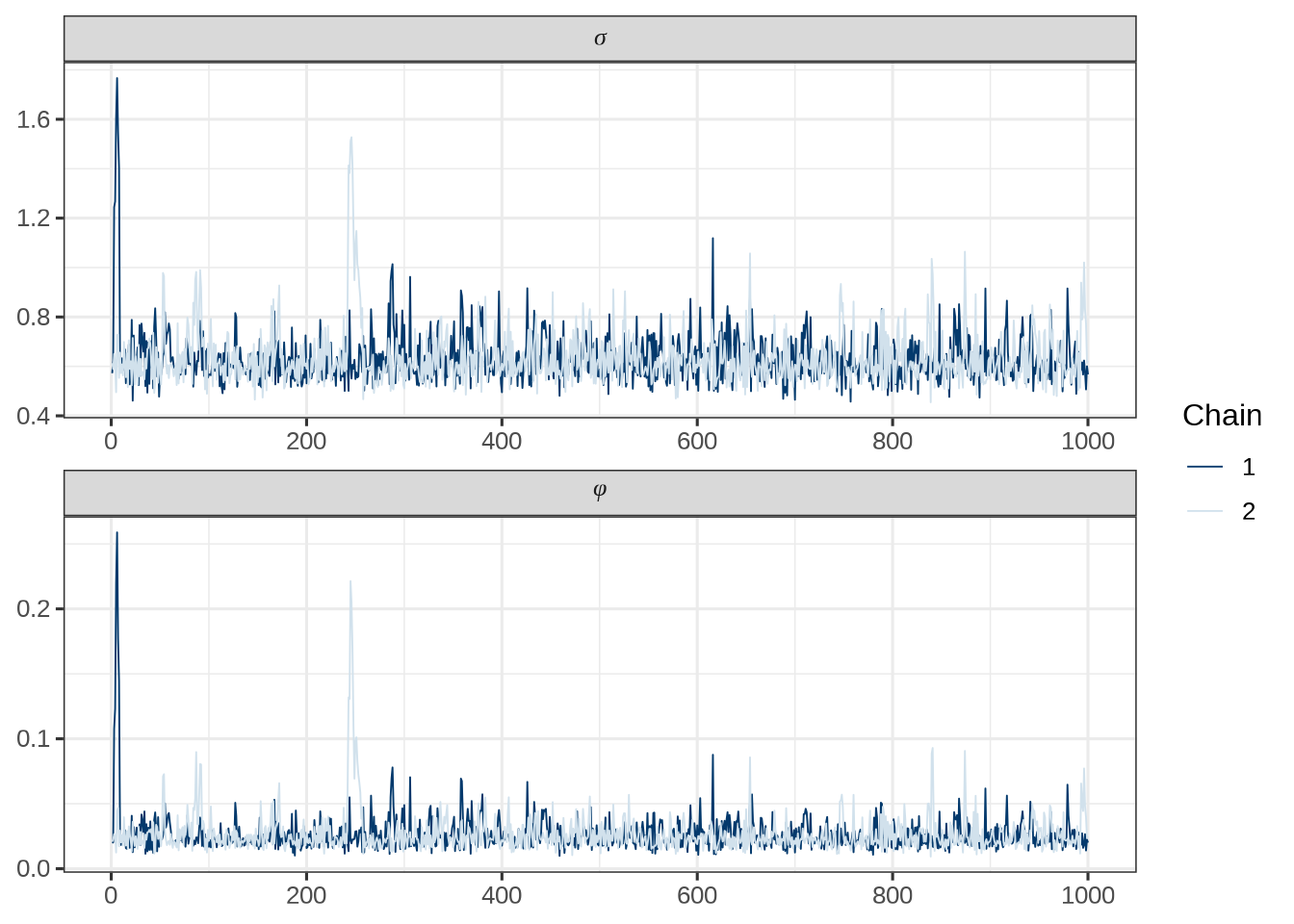
38.3.5 预测分布
核辐射预测模型的 Stan 代码
functions {
  vector gp_pred_rng(array[] vector x2,
                     vector lambda,
                     array[] vector x1,
                     real beta,
                     real sigma,
                     real phi,
                     real delta) {
    int N1 = rows(lambda);
    int N2 = size(x2);
    vector[N2] f2;
    {
      matrix[N1, N1] L_K;
      vector[N1] K_div_lambda;
      matrix[N1, N2] k_x1_x2;
      matrix[N1, N2] v_pred;
      vector[N2] f2_mu;
      matrix[N2, N2] cov_f2;
      matrix[N2, N2] diag_delta;
      matrix[N1, N1] K;
      K = gp_exponential_cov(x1, sigma, phi);
      L_K = cholesky_decompose(K);
      K_div_lambda = mdivide_left_tri_low(L_K, lambda - beta);
      K_div_lambda = mdivide_right_tri_low(K_div_lambda', L_K)';
      k_x1_x2 = gp_exponential_cov(x1, x2, sigma, phi);
      f2_mu = beta + (k_x1_x2' * K_div_lambda);
      v_pred = mdivide_left_tri_low(L_K, k_x1_x2);
      cov_f2 = gp_exponential_cov(x2, sigma, phi) - v_pred' * v_pred;
      diag_delta = diag_matrix(rep_vector(delta, N2));

      f2 = multi_normal_rng(f2_mu, cov_f2 + diag_delta);
    }
    return f2;
  }
}
data {
  int<lower=1> D;
  int<lower=1> N1;
  array[N1] vector[D] x1;
  array[N1] int<lower = 0> y1;
  vector[N1] offsets1;
  int<lower=1> N2;
  array[N2] vector[D] x2;
  vector[N2] offsets2;
}
transformed data {
  real delta = 1e-12;
  vector[N1] log_offsets1 = log(offsets1);
  vector[N2] log_offsets2 = log(offsets2);

  int<lower=1> N = N1 + N2;
  array[N] vector[D] x;

  for (n1 in 1:N1) {
    x[n1] = x1[n1];
  }
  for (n2 in 1:N2) {
    x[N1 + n2] = x2[n2];
  }
}
parameters {
  real beta;
  real<lower=0> sigma;
  real<lower=0> phi;
  vector[N1] lambda1;
}
transformed parameters {
  vector[N1] mu = rep_vector(beta, N1);
}
model {
  matrix[N1, N1] L_K;
  {
    matrix[N1, N1] K = gp_exponential_cov(x1, sigma, phi) + diag_matrix(rep_vector(delta, N1));
    L_K = cholesky_decompose(K);
  }

  beta ~ std_normal();
  sigma ~ inv_gamma(5, 5);
  phi ~ std_normal();

  lambda1 ~ multi_normal_cholesky(mu, L_K);
  y1 ~ poisson_log(log_offsets1 + lambda1);
}
generated quantities {
  vector[N1] yhat;     // Posterior predictions for each location
  vector[N1] log_lik;  // Log likelihood for each location
  vector[N1] RR1 = log_offsets1 + lambda1;

  for(n in 1:N1) {
    log_lik[n] = poisson_log_lpmf(y1[n] | RR1[n]);
    yhat[n] = poisson_log_rng(RR1[n]);
  }

  vector[N2] ypred;
  vector[N2] lambda2 = gp_pred_rng(x2, lambda1, x1, beta, sigma, phi, delta);
  vector[N2] RR2 = log_offsets2 + lambda2;

  for(n in 1:N2) {
    ypred[n] = poisson_log_rng(RR2[n]);
  }
}
准备数据、拟合模型
# 固定漂移项
rongelap_grid_df$time <- 100
# 对数高斯模型
rongelap_poisson_pred_d <- list(
  D = 2,
  N1 = nrow(rongelap), # 观测记录的条数
  x1 = rongelap[, c("cX", "cY")] / 6000,
  y1 = rongelap[, "counts"],
  offsets1 = rongelap[, "time"],
  N2 = nrow(rongelap_grid_df), # 2 维坐标
  x2 = rongelap_grid_df[, c("cX", "cY")] / 6000,
  offsets2 = rongelap_grid_df[, "time"]
)
# 迭代链数目
nchains <- 2
# 给每条链设置不同的参数初始值
inits_data_poisson_pred <- lapply(1:nchains, function(i) {
  list(
    beta = rnorm(1),
    sigma = runif(1),
    phi = runif(1),
    lambda = rnorm(157)
  )
})
# 编译模型
mod_rongelap_poisson_pred <- cmdstan_model(
  stan_file = "code/rongelap_poisson_pred.stan",
  compile = TRUE, cpp_options = list(stan_threads = TRUE)
)
# 泊松模型
fit_rongelap_poisson_pred <- mod_rongelap_poisson_pred$sample(
  data = rongelap_poisson_pred_d,   # 观测数据
  init = inits_data_poisson_pred,   # 迭代初值
  iter_warmup = 500,            # 每条链预处理迭代次数
  iter_sampling = 1000,         # 每条链总迭代次数
  chains = nchains,             # 马尔科夫链的数目
  parallel_chains = 2,      # 指定 CPU 核心数,可以给每条链分配一个
  threads_per_chain = 2,    # 每条链设置一个线程
  show_messages = FALSE,    # 不显示迭代的中间过程
  refresh = 0,              # 不显示采样的进度
  output_dir = "data-raw/",
  seed = 20232023           # 设置随机数种子,不要使用 set.seed() 函数
)
# 诊断信息
fit_rongelap_poisson_pred$diagnostic_summary()
$num_divergent
[1] 0 0
$num_max_treedepth
[1] 0 0
$ebfmi
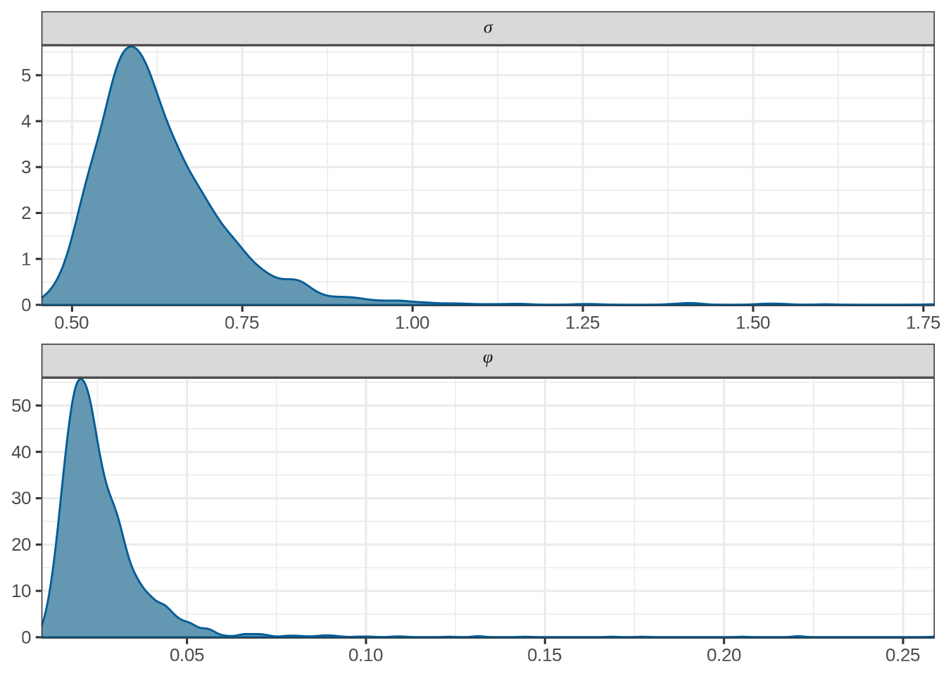
[1] 1.096103 1.065450参数的后验估计
# A tibble: 3 × 10
  variable   mean median     sd     mad     q5    q95  rhat ess_bulk ess_tail
  <chr>     <dbl>  <dbl>  <dbl>   <dbl>  <dbl>  <dbl> <dbl>    <dbl>    <dbl>
1 beta     1.77   1.79   0.145  0.120   1.53   1.97    1.00    1423.     647.
2 sigma    0.638  0.610  0.116  0.0789  0.515  0.851   1.01     855.     474.
3 phi      0.0271 0.0233 0.0152 0.00787 0.0141 0.0513  1.00     763.     539.
模型评估 LOO-CV
Warning: Some Pareto k diagnostic values are too high. See help('pareto-k-diagnostic') for details.
Computed from 2000 by 157 log-likelihood matrix

         Estimate  SE
elpd_loo   -933.7 3.9
p_loo       119.2 2.8
looic      1867.4 7.8
------
Monte Carlo SE of elpd_loo is NA.

Pareto k diagnostic values:
                         Count Pct.    Min. n_eff
(-Inf, 0.5]   (good)       0    0.0%   <NA>
 (0.5, 0.7]   (ok)        18   11.5%   58
   (0.7, 1]   (bad)      110   70.1%   8
   (1, Inf)   (very bad)  29   18.5%   5
See help('pareto-k-diagnostic') for details.
检查辐射强度分布的拟合效果
# 抽取 yrep 数据
yrep <- fit_rongelap_poisson_pred$draws(variables = "yhat", format = "draws_matrix")
# Posterior predictive checks
pp_check(rongelap$counts / rongelap$time,
  yrep = sweep(yrep[1:50, ], MARGIN = 2, STATS = rongelap$time, FUN = `/`),
  fun = ppc_dens_overlay
) +
  theme_classic()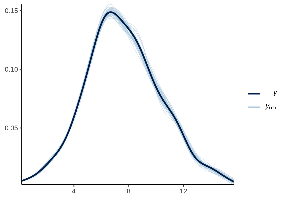
后 1000 次迭代是平稳的,可取任意一个链条的任意一次迭代,获得采样点处的预测值
数据集 rongelap_sf 的概况
Simple feature collection with 157 features and 4 fields
Geometry type: POINT
Dimension: XY
Bounding box: xmin: -6050 ymin: -3430 xmax: -50 ymax: 0
CRS: NA
First 10 features:
counts time geometry lambda yhat
1 75 300 POINT (-6050 -3270) -1.220190 90
2 371 300 POINT (-6050 -3165) 0.183427 361
3 1931 300 POINT (-5925 -3320) 1.842720 1918
4 4357 300 POINT (-5925 -3165) 2.670960 4370
5 2114 300 POINT (-5800 -3350) 1.951680 2136
6 2318 300 POINT (-5800 -3165) 2.053260 2324
7 1975 300 POINT (-5625 -3350) 1.877460 2006
8 1912 300 POINT (-5700 -3260) 1.857760 1940
9 1902 300 POINT (-5700 -3220) 1.815000 1881
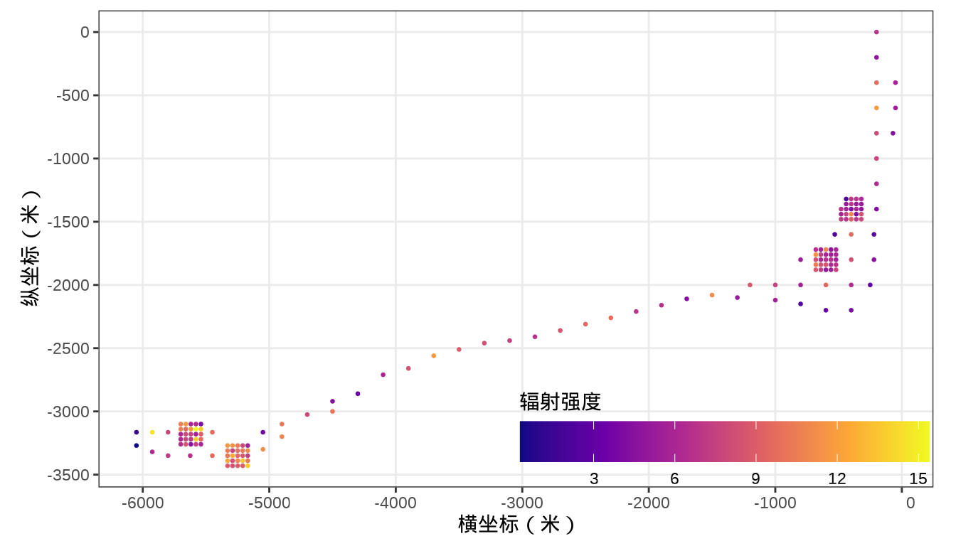
10 1882 300 POINT (-5700 -3180) 1.840230 1837观测值和预测值的情况
   Min. 1st Qu.  Median    Mean 3rd Qu.    Max.
0.250 5.890 7.475 7.604 9.363 15.103 Min. 1st Qu. Median Mean 3rd Qu. Max.
0.300 5.820 7.373 7.609 9.573 15.383 展示采样点处的预测值
代码
ggplot(data = rongelap_sf)+
  geom_sf(aes(color = yhat / time), cex = 0.5) +
  scale_colour_viridis_c(option = "C", breaks = 3*0:5,
    guide = guide_colourbar(
      barwidth = 15, barheight = 1.5,
      title.position = "top" # 图例标题位于图例上方
    )) +
  theme_bw() +
  labs(x = "横坐标(米)", y = "纵坐标(米)", colour = "辐射强度") +
  theme(
    legend.position = c(0.75, 0.1),
    legend.direction = "horizontal",
    legend.background = element_blank()
  )
未采样点的预测
# 后验估计
ypred_tbl <- fit_rongelap_poisson_pred$summary(variables = "ypred", "mean")
rongelap_grid_df$ypred <- ypred_tbl$mean
# 查看预测结果
head(rongelap_grid_df)
cX cY time ypred
1 -5685.942 -3606.997 100 748.5820
2 -5643.145 -3606.997 100 764.2190
3 -5600.347 -3606.997 100 769.1420
4 -5557.549 -3606.997 100 783.6340
5 -5514.751 -3606.997 100 798.8565
6 -5471.953 -3606.997 100 819.4740 Min. 1st Qu. Median Mean 3rd Qu. Max.
0.495 6.194 7.411 7.311 8.531 12.806 转化数据类型,去掉缓冲区内的预测位置,准备绘制辐射强度预测值的分布
代码
# 虚线框数据
dash_sfp <- st_polygon(x = list(rbind(
  c(-6000, -3600),
  c(-6000, -2600),
  c(-5000, -2600),
  c(-5000, -3600),
  c(-6000, -3600)
)), dim = "XY")
# 主体内容
p3 <- ggplot() +
  geom_stars(
    data = rongelap_stars, na.action = na.omit,
    aes(fill = ypred / time)
  ) +
  # 海岸线
  geom_sf(
    data = rongelap_coastline_sfp,
    fill = NA, color = "gray30", linewidth = 0.5
  ) +
  # 图例
  scale_fill_viridis_c(
    option = "C", breaks = 0:13,
    guide = guide_colourbar(
      barwidth = 15, barheight = 1.5,
      title.position = "top" # 图例标题位于图例上方
    )
  ) +
  # 虚线框
  geom_sf(data = dash_sfp, fill = NA, linewidth = 0.75, lty = 2) +
  # 箭头
  geom_segment(
    data = data.frame(x = -5500, xend = -5000, y = -2600, yend = -2250),
    aes(x = x, y = y, xend = xend, yend = yend),
    arrow = arrow(length = unit(0.03, "npc"))
  ) +
  theme_bw() +
  labs(x = "横坐标(米)", y = "纵坐标(米)", fill = "辐射强度") +
  theme(
    legend.position = c(0.75, 0.1),
    legend.direction = "horizontal",
    legend.background = element_blank()
  )

p4 <- ggplot() +
  geom_stars(
    data = rongelap_stars, na.action = na.omit,
    aes(fill = ypred / time), show.legend = FALSE
  ) +
  geom_sf(
    data = rongelap_coastline_sfp,
    fill = NA, color = "gray30", linewidth = 0.75
  ) +
  scale_fill_viridis_c(option = "C", breaks = 0:13) +
  # 虚线框
  geom_sf(data = dash_sfp, fill = NA, linewidth = 0.75, lty = 2) +
  theme_void() +
  coord_sf(expand = FALSE, xlim = c(-6000, -5000), ylim = c(-3600, -2600))
# 叠加图形
p3
print(p4, vp = grid::viewport(x = .3, y = .65, width = .45, height = .45))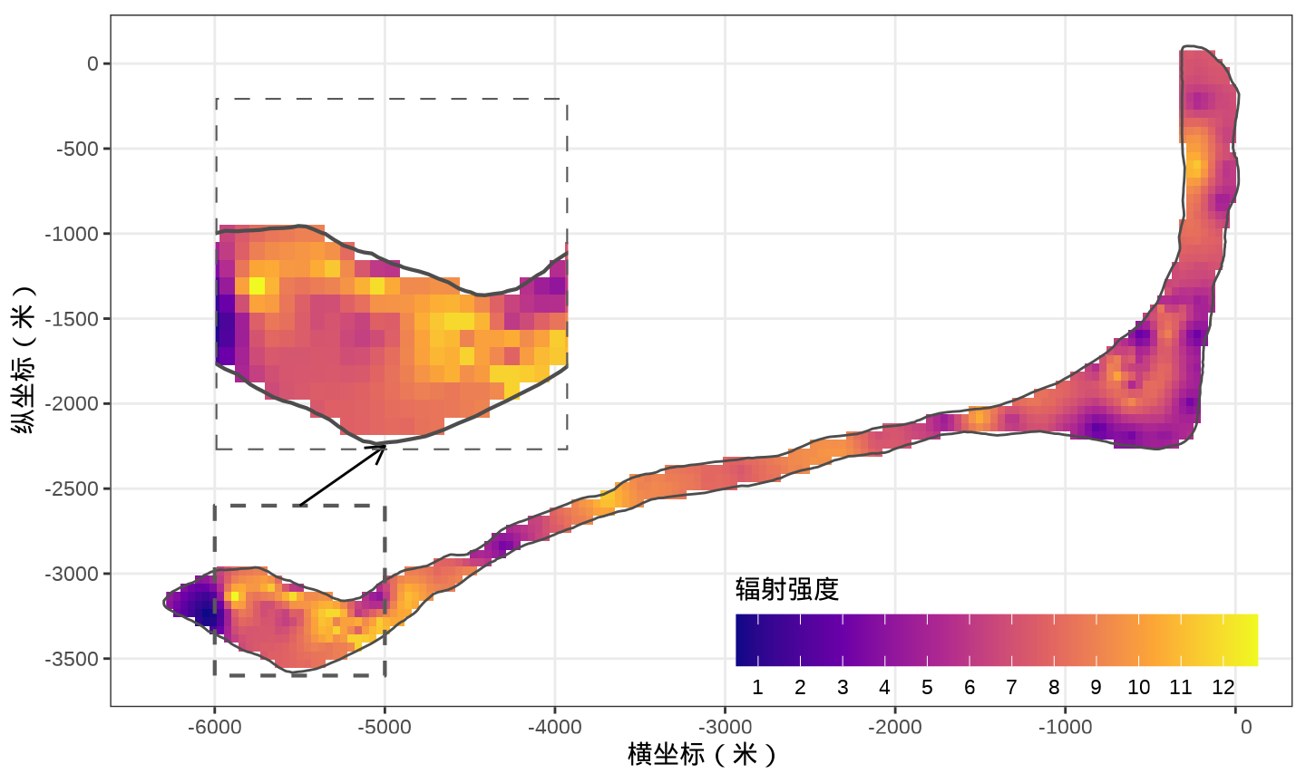
38.4 总结
从模型是否含有块金效应、不同的自相关函数和参数估计方法等方面比较。
library(nlme)
# 高斯分布、指数型自相关结构
fit_exp_reml <- gls(log(counts / time) ~ 1,
  correlation = corExp(value = 200, form = ~ cX + cY, nugget = FALSE),
  data = rongelap, method = "REML"
)
fit_exp_ml <- gls(log(counts / time) ~ 1,
  correlation = corExp(value = 200, form = ~ cX + cY, nugget = FALSE),
  data = rongelap, method = "ML"
)
fit_exp_reml_nugget <- gls(log(counts / time) ~ 1,
  correlation = corExp(value = c(200, 0.1), form = ~ cX + cY, nugget = TRUE),
  data = rongelap, method = "REML"
)
fit_exp_ml_nugget <- gls(log(counts / time) ~ 1,
  correlation = corExp(value = c(200, 0.1), form = ~ cX + cY, nugget = TRUE),
  data = rongelap, method = "ML"
)

# 高斯分布、高斯型自相关结构
fit_gaus_reml <- gls(log(counts / time) ~ 1,
  correlation = corGaus(value = 200, form = ~ cX + cY, nugget = FALSE),
  data = rongelap, method = "REML"
)
fit_gaus_ml <- gls(log(counts / time) ~ 1,
  correlation = corGaus(value = 200, form = ~ cX + cY, nugget = FALSE),
  data = rongelap, method = "ML"
)
fit_gaus_reml_nugget <- gls(log(counts / time) ~ 1,
  correlation = corGaus(value = c(200, 0.1), form = ~ cX + cY, nugget = TRUE),
  data = rongelap, method = "REML"
)
fit_gaus_ml_nugget <- gls(log(counts / time) ~ 1,
  correlation = corGaus(value = c(200, 0.1), form = ~ cX + cY, nugget = TRUE),
  data = rongelap, method = "ML"
)
汇总结果见下表。
| 响应变量分布 | 空间自相关结构 | 块金效应 | 估计方法 | \(\beta\) | \(\sigma^2\) | \(\phi\) | 对数似然值 |
|---|---|---|---|---|---|---|---|
| 高斯分布 | 指数型 | 无 | REML | 1.826 | 0.3172 | 110.8 | -89.07 |
| 高斯分布 | 指数型 | 无 | ML | 1.828 | 0.3064 | 105.4 | -87.56 |
| 高斯分布 | 指数型 | 0.03598 | REML | 1.813 | 0.2935 | 169.7472 | -88.22 |
| 高斯分布 | 指数型 | 0.03312 | ML | 1.828 | 0.2779 | 150.1324 | -86.88 |
| 高斯分布 | 高斯型 | 无 | REML | 1.878 | 0.2523 | 41.96 | -100.7 |
| 高斯分布 | 高斯型 | 无 | ML | 1.879 | 0.25 | 41.81 | -98.62 |
| 高斯分布 | 高斯型 | 0.07055 | REML | 1.831 | 0.2532 | 139.1431 | -84.91 |
| 高斯分布 | 高斯型 | 0.07053 | ML | 1.832 | 0.2459 | 137.0980 | -83.32 |
相比于其他参数,REML 和 ML 估计方法对参数 \(\phi\) 影响很大,ML 估计的 \(\phi\) 和对数似然函数值更大。高斯型自相关结构中,REML 和 ML 估计方法对参数 \(\phi\) 的估计结果差不多。函数 gls() 对初值要求不高,以上初值选取比较随意,只是符合要求函数定义。
对普通用户来说,想要流畅地使用 Stan 框架,需要面对很多挑战。
- 软件安装和配置过程复杂。rstan 包内置的 Stan 版本常低于最新发布的 Stan 版本。
- 编译和运行模型的参数控制选项很多。编译模型,OpenCL 和多线程支持,HMC(NUTS)、L-BFGS 和 VI 三大推理算法的参数设置
- 模型参数先验分布设置技巧高。模型参数的先验对数据的依赖非常高,仅对线性和广义线性模型依赖较小。即使是面对模拟的简单广义线性混合效应模型,抽样过程也发散严重。
- 面对大规模数据扩展困难。以朗格拉普岛的核污染预测任务为例,处理 157 维的积分显得吃力,对 1600 个参数的后验分布模拟和推断低效。
2020 年 Stan 大会 Wade Brorsen 介绍采用 Stan 实现的贝叶斯克里金(Kriging)平滑算法估计和预测各郡县的作物产量。Stan 实现的贝叶斯空间分层正态模型,回归参数随空间区域位置变化,参数的先验分布与空间区域相关,引入大量带超参数的先验分布,运行效率不高,跑模型花费很多时间。假定所有的参数随空间位置变化,模型参数个数瞬间爆炸,跑模型花费 31 天 (Niyizibi, Brorsen, 和 Park 2018)。
Stan 总有些优势吧!
38.5 习题
-
对核辐射污染数据,建立对数高斯过程模型,用 Stan 编码模型,预测全岛的核辐射强度分布。
\[ \begin{aligned} \beta &\sim \mathrm{std\_normal}(0,1) \\ \sigma &\sim \mathrm{inv\_gamma}(5,5) \\ \phi &\sim \mathrm{half\_std\_normal}(0,1) \\ \tau &\sim \mathrm{half\_std\_normal}(0,1) \\ \bm{y} &\sim \mathrm{multivariate\_normal}(\bm{\beta}, \sigma^2 \Sigma+ \tau^2 I) \end{aligned} \]
其中,\(\beta\) 代表截距,先验分布为标准正态分布,\(\sigma\) 代表高斯过程的方差参数(信号),先验分布为逆伽马分布,\(\phi\) 代表高斯过程的范围参数,先验分布为半标准正态分布,\(y\) 代表辐射强度的对数,给定参数和数据的条件分布为多元正态分布,\(\Sigma\) 代表协方差矩阵,\(I\) 代表与采样点数量相同的单位矩阵, \(\tau^2\) 是块金效应。
functions {
  vector gp_pred_rng(array[] vector x2,
                     vector y1,
                     array[] vector x1,
                     real sigma,
                     real phi,
                     real tau,
                     real delta) {
    int N1 = rows(y1);
    int N2 = size(x2);
    vector[N2] f2;
    {
      matrix[N1, N1] L_K;
      vector[N1] K_div_y1;
      matrix[N1, N2] k_x1_x2;
      matrix[N1, N2] v_pred;
      vector[N2] f2_mu;
      matrix[N2, N2] cov_f2;
      matrix[N2, N2] diag_delta;
      matrix[N1, N1] K;
      K = gp_exponential_cov(x1, sigma, phi);
      for (n in 1:N1) {
        K[n, n] = K[n, n] + square(tau);
      }
      L_K = cholesky_decompose(K);
      K_div_y1 = mdivide_left_tri_low(L_K, y1);
      K_div_y1 = mdivide_right_tri_low(K_div_y1', L_K)';
      k_x1_x2 = gp_exponential_cov(x1, x2, sigma, phi);
      f2_mu = (k_x1_x2' * K_div_y1);
      v_pred = mdivide_left_tri_low(L_K, k_x1_x2);
      cov_f2 = gp_exponential_cov(x2, sigma, phi) - v_pred' * v_pred;
      diag_delta = diag_matrix(rep_vector(delta, N2));

      f2 = multi_normal_rng(f2_mu, cov_f2 + diag_delta);
    }
    return f2;
  }
}
data {
  int<lower=1> D;
  int<lower=1> N1;
  array[N1] vector[D] x1;
  vector[N1] y1;
  int<lower=1> N2;
  array[N2] vector[D] x2;
}
transformed data {
  real delta = 1e-9;
}
parameters {
  real beta;
  real<lower=0> phi;
  real<lower=0> sigma;
  real<lower=0> tau;
}
transformed parameters {
  vector[N1] mu = rep_vector(beta, N1);
}
model {
  matrix[N1, N1] L_K;
  {
    matrix[N1, N1] K = gp_exponential_cov(x1, sigma, phi);
    real sq_tau = square(tau);

    // diagonal elements
    for (n1 in 1:N1) {
      K[n1, n1] = K[n1, n1] + sq_tau;
    }

    L_K = cholesky_decompose(K);
  }

  beta ~ std_normal();
  phi ~ std_normal();
  sigma ~ inv_gamma(5, 5);
  tau ~ std_normal();

  y1 ~ multi_normal_cholesky(mu, L_K);
}
generated quantities {
  vector[N2] f2;
  vector[N2] ypred;

  f2 = gp_pred_rng(x2, y1, x1, sigma, phi, tau, delta);
  for (n2 in 1:N2) {
    ypred[n2] = normal_rng(f2[n2], tau);
  }
}
代码中,
gp_exponential_cov表示空间相关性结构选择了指数型,详见 Stan 函数手册中的指数型核函数表示。cholesky_decompose表示对协方差矩阵做 Cholesky 分解,分解出来的下三角矩阵作为多元正态分布的参数,详见 Stan 函数手册中的 Cholesky 分解。multi_normal_cholesky表示基于 Cholesky 分解的多元正态分布。详见 Stan 函数手册中的多元正态分布的 Cholesky 参数化表示。代码
set.seed(20232023)
nchains <- 2 # 2 条迭代链
# 给每条链设置不同的参数初始值
inits_data_gaussian <- lapply(1:nchains, function(i) {
  list(
    beta = rnorm(1),
    sigma = runif(1),
    phi = runif(1),
    tau = runif(1)
  )
})

# 对数高斯模型
rongelap_gaussian_d <- list(
  N1 = nrow(rongelap), # 观测记录的条数
  N2 = nrow(rongelap_grid_df),
  D = 2, # 2 维坐标
  x1 = rongelap[, c("cX", "cY")] / 6000, # N x 2 坐标矩阵
  x2 = rongelap_grid_df[, c("cX", "cY")] / 6000,
  y1 = log(rongelap$counts / rongelap$time) # N 向量
)
# 编码
mod_rongelap_gaussian <- cmdstan_model(
  stan_file = "code/gaussian_process_pred.stan",
  compile = TRUE, cpp_options = list(stan_threads = TRUE)
)

# 对数高斯模型
fit_rongelap_gaussian <- mod_rongelap_gaussian$sample(
  data = rongelap_gaussian_d,   # 观测数据
  init = inits_data_gaussian,   # 迭代初值
  iter_warmup = 500,            # 每条链预处理迭代次数
  iter_sampling = 1000,         # 每条链总迭代次数
  chains = nchains,             # 马尔科夫链的数目
  parallel_chains = 2,      # 指定 CPU 核心数,可以给每条链分配一个
  threads_per_chain = 1,    # 每条链设置一个线程
  show_messages = FALSE,    # 不显示迭代的中间过程
  refresh = 0,              # 不显示采样的进度
  output_dir = "data-raw/",
  seed = 20232023           # 设置随机数种子,不要使用 set.seed() 函数
)

# 诊断
fit_rongelap_gaussian$diagnostic_summary()
# 对数高斯模型
fit_rongelap_gaussian$summary(
  variables = c("lp__", "beta", "sigma", "phi", "tau"),
  .num_args = list(sigfig = 4, notation = "dec")
)

# 未采样的位置的核辐射强度预测值
ypred <- fit_rongelap_gaussian$summary(variables = "ypred", "mean")
# 预测值
rongelap_grid_df$ypred <- exp(ypred$mean)
# 整理数据
rongelap_grid_sf <- st_as_sf(rongelap_grid_df, coords = c("cX", "cY"), dim = "XY")
rongelap_grid_stars <- st_rasterize(rongelap_grid_sf, nx = 150, ny = 75)
rongelap_stars <- st_crop(x = rongelap_grid_stars, y = rongelap_coastline_sfp)

# 虚线框数据
dash_sfp <- st_polygon(x = list(rbind(
  c(-6000, -3600),
  c(-6000, -2600),
  c(-5000, -2600),
  c(-5000, -3600),
  c(-6000, -3600)
)), dim = "XY")
# 主体内容
p3 <- ggplot() +
  geom_stars(
    data = rongelap_stars, na.action = na.omit,
    aes(fill = ypred)
  ) +
  # 海岸线
  geom_sf(
    data = rongelap_coastline_sfp,
    fill = NA, color = "gray30", linewidth = 0.5
  ) +
  # 图例
  scale_fill_viridis_c(
    option = "C", breaks = 0:12,
    guide = guide_colourbar(
      barwidth = 15, barheight = 1.5,
      title.position = "top" # 图例标题位于图例上方
    )
  ) +
  # 虚线框
  geom_sf(data = dash_sfp, fill = NA, linewidth = 0.75, lty = 2) +
  # 箭头
  geom_segment(
    data = data.frame(x = -5500, xend = -5000, y = -2600, yend = -2250),
    aes(x = x, y = y, xend = xend, yend = yend),
    arrow = arrow(length = unit(0.03, "npc"))
  ) +
  theme_bw() +
  labs(x = "横坐标(米)", y = "纵坐标(米)", fill = "辐射强度") +
  theme(
    legend.position = c(0.75, 0.1),
    legend.direction = "horizontal",
    legend.background = element_blank()
  )

p4 <- ggplot() +
  geom_stars(
    data = rongelap_stars, na.action = na.omit,
    aes(fill = ypred), show.legend = FALSE
  ) +
  geom_sf(
    data = rongelap_coastline_sfp,
    fill = NA, color = "gray30", linewidth = 0.75
  ) +
  scale_fill_viridis_c(option = "C", breaks = 0:12) +
  # 虚线框
  geom_sf(data = dash_sfp, fill = NA, linewidth = 0.75, lty = 2) +
  theme_void() +
  coord_sf(expand = FALSE, xlim = c(-6000, -5000), ylim = c(-3600, -2600))
# 叠加图形
p3
print(p4, vp = grid::viewport(x = .3, y = .65, width = .45, height = .45))